This example contains 'certain' detections in all surveys, so it might correspond to a study where all surveys were done with the same method, but a subset of detections were 'verified' to determine if they were recorded correctly.

This software was developed to enable estimation of the proportion of area of occupied (PAO), or similarly the probability a site is occupied, by a species of interest according to the model presented by MacKenzie et al. (2002) 1.
Typically, species are not guaranteed to be detected even when present at a site, hence the naïve estimate of PAO given by:
                # sites where species detected
         PAO = --------------------------------
                    total # sites surveyed
will underestimate the true PAO. MacKenzie et al. (2002) propose that by repeated surveying of the sites, the probability of detecting the species can by estimated which then enables unbiased estimation of PAO. This model has been extended by MacKenzie et al. (2003)2 that also enables estimation of colonization and local extinction probabilities. These models are briefly discussed here.
Currently, there are many types of models can be fit to detection/nondetection data within Program PRESENCE.
Program PRESENCE has been run sucessfully on MAC's (using BootCamp, Wine or Parallels) and Linux PC's (using Wine).
Note: From time to time, it's a good idea to check to make sure you
have the latest version of PRESENCE. This can be done automatically in the 'Tools'
menu. This might prevent the case of reporting a bug which has already
been fixed.
Running the program
Overview: The program can get input data (presence/absence data and site/sample covariate data) from a few different sources.
The 2nd option above is the recommended choice since most spreadsheet programs will automatically backup the data as it is entered. In case the power fails, you might be able to retrieve previously entered data. If you choose the first option, you should periodically save your work.
Once the data are entered into the program, it must be saved (use menu option File/Save) in order to build and run models. The saved file will have an extension (last 3 characters of filename) of "pao". This file will contain both presence/absence data and site and sample covariate data.
To build and run models, a 'project-folder' is created by the program. This file will contain the results of each model in separate files, as well as the input (pao) file and summary results (pa3) file.
To start a new analysis, Select 'File/New project' from the menus. A form will
appear which will hold the information about the analysis, including title,
filenames, data-type, and numbers of sites/occasions/covariates. At this
point, you may use a previously-created input file (something.pao) by clicking
the 'select file' button, or go to the input screen by clicking the 'Input
form' button. Clicking the 'select file' button allows you to navigate to the
folder containing the input file and select the file. Clicking the 'Input
Form' button displays a new form with a tabbed spreadsheet-like interface.
Input Form
To enter data into this form, click on the first element (site 1, sample #1), and enter '1' (without quotes) if the species was detected at site 1, sample #1, '0' if the species was not detected, or '-' if this site was not sampled. The 'Tab' key will move the cursor to the next sample (or use the mouse) where you can enter the data for site 1, sample 2.
If your data is already entered in a spreadsheet program, you can open that program, select all the site/sample data (no headers or other fields), and click 'Edit/Copy' from the menus. Then, go back to PRESENCE, and click the 'Edit/Paste values' from the menu. If your spreadsheet contains sitenames in the first column, you can include these in the selection-edit-copy, then select 'Edit/Paste w/sitenames' in the PRESENCE menu.
If you have covariate data. (e.g., weather or effort data), you can enter these by changing the number of covariates in the appropriate box, then clicking the appropriate tab and entering data as was done with the presence/absence data.
Also included on the input form is an option of simulating data (single-season model only at this time). This is useful if you are just trying the program and have no data, or if you would like to design an experiment and would like to know how many sites/samples are needed to get a desired level of precision (although, program GENPRES will do a much better job). Both presence/absence data and covariate data may be simulated. (A much more extensive program for simulating data is program GENPRES.)
To simulate presence/absence data, click the 'Presence/Absence data' tab, then click 'Generate data' under the 'Simulate' menu. You will be prompted for a value of psi, then values of p (one for each survey or occasion). Optionally, you can enter the value of psi as a linear function of the first covariate (e.g., 0.75 - 0.1*X1), however, you must first simulate the covariate data. Values of p should be separated by commas with no spaces in between.
To simulate covariate data, click the 'Site Covars' tab, then click 'Generate data' under the 'Simulate' menu. You will then be prompted for a mean covariate value, followed by a standard error. Binomial data can be generated by entering '-99' for the mean, followed by the binomial probability (p) for the standard error.
Once the data are entered (or simulated), click 'File/Save' from the menu, then click 'File/Close'. This is an important step, as PRESENCE will not be able to use data in the form unless it has been saved.
Next, click the 'select file' button on the 'enter specifications' form, and use the Windows file selector to navigate to the folder where the saved file resides and select the file. If you've used the input data form and saved the file from the file menu, the input filename and results filename will already be entered for you.
Once you've entered the input (pao) and results (pa3) filenames, click the 'OK' button to create the PRESENCE project folder. This will close the specification window and open a 'Results summary' window. You are now ready to compute estimates under pre-defined models, or build your own 'Custom' model.
The species may or may not be detected during a survey and is not falsely detected when absent (except false-positive model). The resulting detection history for each site may be expressed as T vectors of 1's and 0's, indicating detection and nondetection of the species respectively. We denote the detection history for site i at primary sampling period j as Xi,j, and the complete detection history for site i, over all primary periods, as Xi. The single season model results when K=1, and the multiple season model for K>1.
MacKenzie et al. (2002)1 present a model for estimating the site occupancy probability (or PAO) for a target species, in situations where the species is not guaranteed to be detected even when present at a site. Let ψ be the probability a site is occupied and p[j] be the probability of detecting the species in the jth survey, given it is present at the site. They use a probabilistic argument to describe the observed detection history for a site over a series of surveys. For example the probability of observing the history 1001 (denoting the species was detected in the first and fourth surveys of the site) is:
ψ x p[1](1-p[2])(1-p[3])p[4].
The probability of never detecting the species at a site (0000) would therefore be,
ψ x (1-p[1])(1-p[2])(1-p[3])(1-p[4]) + (1-ψ),
which represents the fact that either the species was there, but was never detected, or the species was genuinely absent from the site (1-ψ). By combining these probabilistic statements for all N sites, maximum likelihood estimates of the model parameters can be obtained.
The model framework of MacKenzie et al. (2002) is flexible enough to allow for missing observations: occasions when sites were not surveyed. Missing observations may result by design (it is not logistically possible to always sample all sites), or by accident (a technicians vehicle may breakdown enroute). In effect, a missing observation supplies no information about the detection or nondetection of the species, which is exactly how the model treats such values.
The model also enables parameters to be function of covariates. For example, occupancy probability may be a function of habitat, while detection probability is a function of environmental conditions such as air temperature. The model therefore allows relationships between occupancy state and site characteristics to be investigated. Covariates are entered into the model by way of the logistic model (or logit link).
A key assumption of the single season model is that all parameters are constant across sites. Failure of this creates heterogeneity. Unmodeled heterogeneity in detection probabilities will cause occupancy to be underestimated. If there is unmodelled heterogeneity in occupancy probabilities, then it is believed that the estimates will represent an average level of occupancy, provided detection probabilities are not directly related to the probability of occupancy.
Another major assumption of the MacKenzie et al. (2002) model is that the occupancy state of the sites does not change for the duration of the surveying. Situations where this may be violated, for instance, would be for species with large home ranges, where the species may temporarily be absent from the site during the surveying. If this process of temporary absence from the site may be viewed as a random process, (e.g., the species tosses a coin to decide whether it will be present at the site today), then this assumption may be relaxed. However, this will alter the interpretation of the model parameters ("occupancy" should be interpreted as "use" and "detection" as "in the site and detected"). More systematic mechanisms for temporary absences may be more problematic and create unknown biases. Although, users are reminded that the model assumes closure of the sites at the species level, not at the individual level, so there may be some movement of individuals to/from sites without overly affecting the model.
There are 6 predefined models that users can run. The "groups" refer to the number of (unknown) groups in the population of occupied sites with different detection probabilities. For instance, "Two Groups" suggest there are 2 types of sites where species have different detection probabilities (perhaps related to species abundance, low or high, say), however group membership is unknown. Finite mixture-models are used to model these unknown groups by introducing parameters representing the probability of being in each group (see Pledger 20003, and references therein for details), and this is one approach to allow for heterogeneous detection probabilities. The "Single Group" model is the one discussed by MacKenzie et al. (2002). In each case, detection probabilities (p) may be specified as constant across surveys, or survey specific.
For new users of the program, I'll start with the single-season data-type and describe the process of building/running models. Later, I'll describe how to run the other data-types, although you might be able to skip that part. For the single-season data-type, I can't think of a situation where you would not want to run some of the pre-defined models. To run one of these models, click 'Run/Analysis' from the menus. A form will appear which allows you to pick one of the pre-defined models, or build a custom model. Also on the form are self-explanatory options for the analysis. The pre-defined models include the following models:
| model | description |
|---|---|
| 1 group, constant p | species at all sites/samples are detected with a single probability, p. |
| 1 group, survey-specific p | survey-specific detection probability at all sites, p(1)-detection prob for 1st survey, p(2)=detection prob. for 2nd survey, ... |
| 2 groups, constant p | There are two groups of sites where the species has different detection probabilities, p1, p2, and the proportion of sites which have detection probability of p1 = α | 2 groups, survey-specific p | There are two groups of sites where the species has different detection probabilities at each survey, p1(1), p2(1),p1(2), p2(2),... and the proportion of sites in group 1 = α |
| 3 groups, constant p | There are three groups of sites where the species has different detection probabilities, p1, p2 and p3, the proportion of species which have detection probability of p1 = α1 and the proportion of species which have detection probability of p2 = α2 (the remaining proportion have detection probability, p3. | 3 groups, survey-specific p | There are three groups of sites where the species has different detection probabilities at each survey, p1(1), p2(1),p1(2), p2(2),... and the proportion of sites in group 1 = α1, group 2=α2. |
Program PRESENCE allows you to define models which are not included in the pre-defined model set. To allow flexibility, models are defined by using a 'design-matrix'. This design-matrix can be thought of as a translation-table which transforms real-estimated parameters to/from the model parameters (ψ, and p(i)).
In the design-matrix, the real-estimated parameters are represented by the columns, and the model parameters are represented by the rows. As an example, let's look at building a custom model which is equivalent to the first pre-defined model. When you click 'Run/Analysis', then click 'custom model', the pre-defined model names disappear, and a design-matrix form appears. This form contains a tab for the occupancy model parameter (psi), and a tab for the detection model parameters (p1,p2,p3,p4). If you click the 'occupancy' tab, there will be a spreadsheet with 1 row (psi) and 1 column (a1). The real-estimated parameter is 'a1' and the model parameter is psi, which is computed as psi = 1 * a1. If you click the 'Detection' tab, a spreadsheet will appear which contains 4 rows and 1 column. By default, the model parameter p1, will be computed as: p1 = 1 * b1. The model parameters p2, p3, and p4 will also be computed as: p2 = 1 * b1, p3 = 1 * b1, and p4 = 1 * b1. So, the program will estimate 1 parameter, a1, which will yield a value for psi, and 1 parameter, b1, which will yield values for p1, p2, p3, and p4. This is equivalent to the first pre-defined model. To build a model which is equivalent to the second pre-defined model (1 group, survey-specific P), we need different real-estimated parameters for each detection probability, p1, p2, p3, and p4. To do this, we need to add 3 more columns to the spreadsheet. Click 'Edit/Add cols' from the menus and enter '3' when asked how many columns to add. The spreadsheet should now contain 4 rows and 4 columns. Now, we need to change the numbers in the spreadsheet so that:
p1 = 1 * b1
p2 = 1 * b2
p3 = 1 * b3
p4 = 1 * b4.
Click 'Init/Full Identity' from the menus and the spreadsheet will be filled with 1's on the diagonal, and zeros elsewhere. So, reading the rows of the spreadsheet,
p1 = 1 * b1 + 0 * b2 + 0 * b3 + 0 * b4.
p2 = 0 * b1 + 1 * b2 + 0 * b3 + 0 * b4.
p3 = 0 * b1 + 0 * b2 + 1 * b3 + 0 * b4.
p4 = 0 * b1 + 0 * b2 + 0 * b3 + 1 * b4.
We now have 5 real-estimated parameters (a1,b1,b2,b3,b4), which will be used to compute 5 model parameters (psi,p1,p2,p3,p4). This is equivalent to the second pre-defined model (1 group, survey-specific P).
p1 = 1 * b1 + 0 * b2.
p2 = 1 * b1 + 0 * b2.
p3 = 0 * b1 + 1 * b2.
p4 = 0 * b1 + 1 * b2.
So, the detection spreadsheet would contain 4 rows, and 2 columns (b1,b2) and would look like this:
| . | b1 | b2 |
|---|---|---|
| p1 | 1 | 0 |
| p2 | 1 | 0 |
| p3 | 0 | 1 |
| p4 | 0 | 1 |
In this example, suppose detection probabilities, p(i), are hypothesized to be increasing by a constant amount over the surveys. So, the second detection probability would be equal to the first detection probability plus a constant (X), and the third would be equal to the first + 2*X, and the last detection probability would be equal to the first + 3*X. We would need 2 real-estimated parameters (first detection probability, and X) to compute the 4 model detection parameters. Here is how to write the formulae for the p's:
p1 = 1 * b1 + 0 * b2.
p2 = 1 * b1 + 1 * b2.
p3 = 1 * b1 + 2 * b2.
p4 = 1 * b1 + 3 * b2.
So, the detection spreadsheet would contain 4 rows, and 2 columns (b1,b2) and would look like this:
| . | b1 | b2 |
|---|---|---|
| p1 | 1 | 0 |
| p2 | 1 | 1 |
| p3 | 1 | 2 |
| p4 | 1 | 3 |
p(site i, survey j) = 1*b1 + X(i,j)*b2
where X(i,j) is the value of the sample-covariate at site i, sample j. Here, p(i,j) is equal to a base detection probability, (intercept), (1*b1) plus an effect (b2) of the covariate, X(i,j). If b2=0 then there is no effect of the covariate (p=constant). If b2>0 then there is a positive effect of the covariate (higher covariates yield higher p's), and if b2<0 then there is a negative effect of the covariate (higher covariates yield lower p's).
If you had two covariates for each site/sample, you could compute p as:
p(site i, survey j) = 1*b1 + X(i,j)*b2 + Y(i,j)*b3
where Y(i,j) is the value of the 2nd covariate at site i, sample j. The detection design matrix for the case with 2 covariates would look like this:
| . | b1 | b2 | b3 |
|---|---|---|---|
| p1 | 1 | X | Y |
| p2 | 1 | X | Y |
| p3 | 1 | X | Y |
| p4 | 1 | X | Y |
To run this type of model, click 'Run/Analysis', add columns for the covariates, then, instead of entering '1' in the cells, click on the first cell in a column, and select the covariate name from the 'Init' menu.
Now seems like a good time to run through an example. Start program PRESENCE and select 'File/New Project' from the menus. When the 'Enter Specifications' form appears, click the 'Input Data Form' button.
The input data form will contain only 1 tab, for the presence/absence data. We're going to simulate some data in this form. Let's assume we're dealing with a species which has an occupancy rate (ψ) of 0.60 (60% of areas contain at least 1 individual of the species). Also, assume/pretend detection probability is lousy in the beginning, p(1)=0.2, and gets better on each successive sample, p(2)=.4, p(3)=.6, p(4)=.8. This is enough information to generate data for the single-season data-type. To generate presence/absence data, select 'Generate data' from the 'Simulate' menu and enter ψ (0.6) when prompted. Next, enter '0.2,0.4,0.6,0.8' when prompted for the detection probabilities (p) and the table will clear and be filled with randomly generated presence/absence data with those parameters. Click 'File/Save as' and save the file with the name, 'simdata1.pao'. When asked about using the last column for the frequency, click 'No', and enter something for a title. Then, click 'File/Close'.
Next, click the 'Click to select file' button and select the simulated data file we just created (simdata1.pao). The program will fill in the boxes for the filename and results filename. Enter 'simulated data w/ psi=.6, p=.2,.4,.6,.8' in the title box, and click the 'OK' button.
You should see an empty results browser at this point. To run the first pre-defined model, click 'Run/Analysis:single season' from the menus. For the pre-defined models, the program automatically fills in the model name. This name can be anything, but it's best to make it something easily recognized. (I'll describe a common convention for naming later.) In the 'Model' box, you'll see that 'pre-defined' is already selected, and 6 pre-defined models are listed (with the first one selected). Let's start with this model, but first check the 'list data' option. Click 'list-data', then click the 'OK to run' button.
Once you click the 'OK to run' button, you might see another window flash by (perhaps not if you have a fast computer), then a dialog box appears with a short summary of the results of that model. Click 'Yes' to include the output of that model in the results browser. (You might click 'No' in the case where you accidentally run a model which was previously run.) After clicking 'Yes', the summary information from that model is displayed in the results browser.
To view the estimates of psi, and p from this model, use the mouse to position the cursor over the name of the model, '1 group, Constant P', then click with the right mouse button. A pop-up menu will appear. Position the mouse over 'View model output' and click with the left mouse button. This will cause a Notepad window to appear with the results. Look at the output and note the estimates of ψ(Psi), and p. (I got .7267, and .4300, but yours will be different.)
Next, let's run another pre-defined model - one with survey-specific p's. Close the notepad window with the results, then click 'Run/Analysis:single season' from the menus. Click '1 group, survey-specific p' in the 'Model' box (note model name changed for you), then click 'OK to run'. Click 'Yes' to include the results of this model in the results browser, then position the mouse over the model name, right-click, then left-click 'view model output'. In the notepad window, note ψ (Psi), and p(1),p(1),p(3) and p(4). With such a small number of sites and surveys, estimates may be very different from the true values (ψ=.6 , p=.2,.4,.6,.8).
01011Here, the species was detected at the 2nd, 4th and last samples (segments of transect line), but not detected at the 1st and 3rd samples. The probability of this history would be represented by:
ψ[(1-θ1)θ2+θ1(1-p1)θ'2] p2[(1-θ'3)θ4+ θ'3(1-p3)θ'4] p4θ'5p5
In this model, we assumed that the species was not locally present before the first sample (first θ is not θ'), when in reality, the first segment might be one where the species was locally present in the previous segment. In this case, we would want the first θ to be a value between θ and θ'. The value should be the expected value (of local presence) you would get if you randomly picked a survey from all surveys. So, when the spatial dependence model is chosen, there is an option to use the same θ1 for all surveys, or use an 'average' of θs and θ's for the first survey of each site.
When this model is chosen, the θ parameters will appear in the design matrix window, in the same tab as the occupancy (ψ) parameter. This model is described in Hines (2010)11
***New Spatial Dependence Model update ***
A few changes have been made to this model, allowing more flexibility. First, instead of assuming the first segment is at a boundary and the previous segment is unoccupied, we can estimate the proportion of sites where the segment before the first segment is occupied. This proportion parameter is named 'thta0pi'. So, if all sites start out at a boundary (eg., river) and occupancy is impossible before the 1st segment, this new parameter should be estimated to be zero. As with other parameters in PRESENCE, you can fix this parameter if you know that all sites start at a boundary. This would be equivalent to the default model (theta option unchecked) in the old version.
If sites don't start at a boundary, you can either let PRESENCE estimate the parameter, thta0pi, or fix the parameter to a specific value, using the usual 'fix parameters' boxes. In order to generate a model that is equivalent to the option, 'theta0 not equal to rest of thetas' in the old version, the string, 'eq.' can be entered into the fixed parameter box for thta0pi. When this is done, thta0pi is computed using the values of θ and θ' in the likelihood function. Since it is computed from other parameters and not estimated on it's own, there is no need for a Beta parameter corresponding to it in the design matrix. So, the design matrix for thta0pi should contain only the column with the name 'thta0pi' (and the other column deleted).
Note: The option to compute θ1 based on the other θs and θ's assumes that the population is in 'equilibrium'. The new version estimates this proportion without that assumption, so it would be a better choice than trying to replicate the old version.
Here is the new probability structure for the detection history listed above (01011), using the new parameter:
ψ[(1-π)(1-θ1)θ2+ π(1-θ'1)θ2+ (1-π)θ1(1-p1)θ'2+ πθ'1(1-p1)θ'2] p2[(1-θ'3)θ4+ θ'3(1-p3)θ'4] p4θ'5p5
Another update to this model allows the theta's to be segment-specific. This may be possible if the detection parameters (p) are constant among segments. This model isn't identifiable (no single solution for parameters) if both theta's and detection probabilities are allowed to be segment-specific.
Parameters:
Data input for this model is as follows:
site1  h1 h2 h3...
site2  h1 h2 h3...
site3  h1 h2 h3...
:
:
where
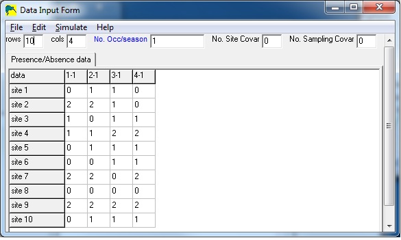
In the sample input below, there are 10 sites and 4 surveys.
This example contains 'certain' detections in all surveys, so it might correspond
to a study where all surveys were done with the same method, but a subset of detections
were 'verified' to determine if they were recorded correctly.
For example, if there are 3 surveys with 'certain' and 'uncertain' detections in each survey, the input detection-history data would contain 6 columns. Columns 1,3,5 would contain uncertain detections in each of the 3 surveys (0=not detected, 1=detected). Columns 2,4,6 would contain certain detections (0=not detected, 2=detected). As far as PRESENCE is concerned, there are 6 surveys, but you will know that there are really only 3 surveys, with two methods per survey.
In the sample below, there are 10 sites and 6 surveys, with the implication that
surveys 1,3,5 are uncertain detections and surveys 2,4,6 are certain
detections.
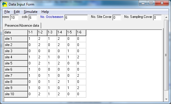
Notice that columns 1,3,5 only contain 0's and 1's, and columns 2,4,6 only
contain 0's and 2's.
When building the model, the detection design matrix will now contain 6 detection probabilities (p11), 6 false-positive probabilites (p10), and 6 'certainty probabilities' (b). Since there cannot be any false-positive detections in surveys 2,4,6, those p10's need to be fixed to zero (p10(2)=0, p10(4)=0, p10(6)=0). Also, since there are no certain detections in surveys 1,3,5, those b's need to be fixed to 0 (b(1)=0, b(3)=0, b(5)=0).
The design matrix and fixed-parameters windows would look like this:
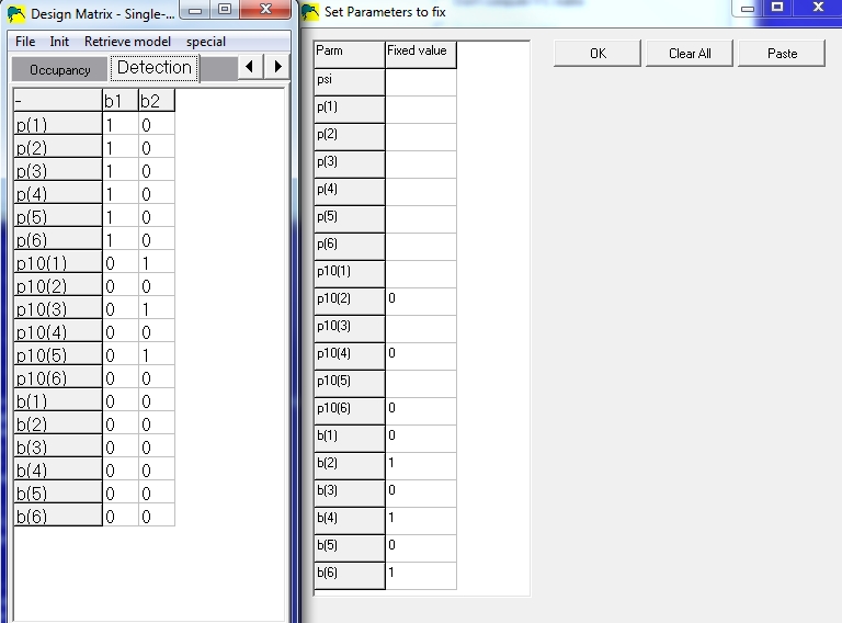
Notice that any parameter which is fixed (right window) contains all zeros for
that row
in the design matrix window (left window). This example design matrix shows a model
where detection probabilities are the same for both methods (p(odd)=p(even)), which
is probably not very realistic. If the methods are drastically different, one would expect
the detection probabilites to be different and model the p's differently.
Parameters:
Parameters:
An alternate parameterization was developed which only uses conditional probabilities as parameters, which is more numerically stable. The parameters are:
ψB = ψA*ψBA+(1-ψA)*ψBa
φ = ψA*ψBA/(ψA*ψB)
Parameters:
Data input for this model is as follows:
site1  h1,1 h1,2 h1,3... h2,1 h2,2 h2,3...
site2  h1,1 h1,2 h1,3... h2,1 h2,2 h2,3...
site3  h1,1 h1,2 h1,3... h2,1 h2,2 h2,3...
:
:
where hi,j = 1 if detection at site for survey i, method j; hi,j = 0 if no detection
Additionally, the number of methods per survey is specified in the 'No. Occ/season' input box, when entering data.
In the sample input below, there are 10 sites, 2 surveys and 2 methods per survey.
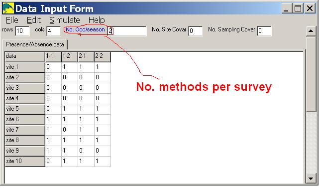
Notice that the column labels (1-1,1-2,2-1,2-2) indicate survey number and method number.
Parameters:
Another way of parameterizing this model is as follows:
This model is more general than the first parameterization, but needs constraints like the one mentioned above in order to be identifiable. To use this parameterization in PRESENCE, treat it like multi-season-multi-state analysis with only one season.
Parameters:
For example, if the detection history 101 000 was observed at a site (denoting the species was detected in the first and third survey of the site in the first season; not detected otherwise), the probability of this occurring could be expressed as;
ψ x p1,1(1-p1,2)p1,3 x {(1-ε1) (1-p2,1) (1-p2,2) (1-p2,3) + ε1}.
This represents the fact that after the first season, the species may have not gone locally extinct (1-ε1), but was undetected by the surveying, or the species did go locally extinct (ε1) between the first and second seasons.
The model may also be reparameterized in terms of ψt and εt; or ψt and γt, as in some situations this may be a more meaningful parameterization (in terms of overall occupancy) than in terms of the underlying processes. As in the single season model, parameters may be functions of covariates using the logit link.
Note this model does not allow for a so-called "rescue effect", where the local extinction of a colony is "rescued" by the re-colonization of the site before the unoccupied site can be observed (i.e., the site becomes unoccupied then re-occupied all between a single season). Such an effect is sometimes included in metapopulation models, however while a rescue effect is biologically plausible, it can not be estimated (without some potentially unrealistic strict assumptions) from the type of data we are considering here, nor from the type of data often collected in metapopulation studies. The main argument for not including a rescue effect is: why should the rescue of the colony be limited to an arbitrary single event, when possibly there may be a number of opportunities between two seasons for the rescue to occur? To reduce the possibility of having unobserved changes in the occupancy state of sites, the sampling scheme should be designed to reflect the appropriate time scale of the system under study.
ψ2 = ψinitial*(1-ε1) + (1-ψinitial)*γ1
ψ3 = ψ2*(1-ε2) + (1-ψ2)*γ2
ψ4 = ψ3*(1-ε3) + (1-ψ3)*γ3
 :         :        :            :        :
Sometimes, it is desirable to model seasonal occupancy as a function of some covariates. Since seasonal occupancy is computed from εi and γi, this cannot be done with these parameters.
An alternate parameterization in PRESENCE uses k occupancy parameters, k-1 extinction parameters, and T detection parameters. The k-1 colonization parameters are then computed from the seasonal ψ's and ε's by solving the above equations for γi.
           ψ2 - ψinitial*(1-ε1)
 γ1 = ---------------------------------
                 (1-ψinitial)
By selecting this parameterization, it's now possible to build a model
where seasonal occupancy (ψi) is a function of a seasonal covariate.
Similarly, we could have estimated the colonization parameters and computed the extinction parameters. This parameterization is sometimes useful if the above parameterization fails to converge on reasonable estimates.
Finally, PRESENCE can model extinction and colonization in such a way that the proportion that go locally extinct is the same as the proportion that don't colonize (ε=1-γ).
Parameters:
Parameters:
If you're willing to assume that all sites are 'neighbors' of each other (i.e., if the individual organisms can move anywhere within the study area), then this model can be run by simply using psi1 as a covariate name in the design matrix. When PRESENCE goes to compute colonization or extinction, it will compute occupancy in season t-1 and use that value as a covariate in computing colonization/extinction in season t.
In the case where it is desired to define neighbors specifically for each site, PRESENCE can read a file which defines the neighbors of each site. This file should be a text file containing 1's and 0's where 1 denotes that site s is a neighbor of site r. The format of the file is rows of contigous 1's and 0's, one row for each focal site. Each row should contain a string of k characters (where k = number of sites in the study area). For example if there were 10 sites, the neighbor file might look like this:
 0100000000
 1000000000
 0001100000
 0010100000
 0011000000
 0000001111
 0000010111
 0000011011
 0000011101
 0000011110
In this example, sites 1 and 2 are neighbors of each other, sites 3,4,5 are neighbors, and sites 6-10 are neighbors. So, if colonization between seasons t-1 and t is modeled as a function of average neighborhood occupancy at time t-1, colonization for site 2 in season t will be a function of the average occupancy for sites 1 and 2 in season t-1.
In some cases, sites may not all be of the same size or habitat quality. In these cases, it would be preferable to weight the average occupancy of neighboring sites by a value indicating the size/quality of each neighboring site. For example, if all sites except site 5 are nearly the same size, but site 5 is twice as large as the other sites, we would want the occupancy for site 5 to have more influence on colonization/extinction of other sites than the occupancy of other sites. So, the neighbor file would be:
 0100000000 1.0
 1000000000 1.0
 0001100000 1.0
 0010100000 1.0
 0011000000 2.0
 0000001111 1.0
 0000010111 1.0
 0000011011 1.0
 0000011101 1.0
 0000011110 1.0
In this example, sites 3,4,5 are neighbors, but the average occupancy used in the computation of colonization for those sites will be computed as:
logit(γsite4,t) = β0 + β1*Xsite4,t-1+...
where X is the auto-logistic covariate and is computed as:
Xsite4,t-1 = (Wsite3 * ψsite3,t-1 + Wsite5 * ψsite5,t-1) / (Wsite3 + Wsite5 )
Using the weights in the example:
Xsite4,t-1 = (1.0 * ψsite3,t-1 + 2.0 * ψsite5,t-1) / (1.0 + 2.0)
(note: X = auto-logistic covariate and W = weight.)
If PRESENCE finds this auto-logistic covariate name, 'psi1', in the design matrix, it will ask for a neighbor text file. If you don't specifiy a file, PRESENCE will assume all sites are neighbors of each other and all have equal weight (as described initially). If a file is specified, the filename will be saved in the results file (*.pa3), and will be used in all future auto-logistic models. If the file is specified and does not contain a column of weights, all sites will be assumed to have equal weight.
Parameters:
Another way of parameterizing this model is as follows:
So, the first parameterization assumes that there are only 3 occupancy states:
Input data consists of the following codes:
0=species not detected at site, habitat state=A,
1=species detected at site, habitat state=A,
2=species not detected at site, habitat state=B,
3=species detected at site, habitat state=B.
Parameters:
Multi-season Two-Species Model
This is an extension of the two-species model (MacKenzie et al., 2004)
16allowing the
computation of occupancy, colonization, extinction and detection
parameters of two species along
with conditional probabilities when the
other species is present or detected.
Parameters:
Alternate Input for 2-species model-
Instead of repeating each site for each species, the following
codes can be used for this model:
********* Input Data summary *******
Number of sites                = 100
Number of sampling occasions   = 5
Number of missing observations = 0
Data checksum = 24240

Naive occupancy estimate       = 0.7266

NSiteCovs-->0
NSampCovs-->0

Predefined Model: Detection probabilities are NOT survey-specific

Number of groups               = 1
Number of parameters           = 2
Number of function calls           = 69
-2log(likelihood)              = 616.330857
AIC                            = 620.330857
Proportion of sites occupied    (Psi)   = 0.7500 (0.0465)

Detection probabilities         (p):
  grp   srvy      p            se(p)
  ---   ----   ---------    -----------
   1      1    0.500000     ( 0.028194)

Variance-Covariance Matrix
   psi    p(G1)
 0.0022 -0.0002
-0.0002  0.0008
------------------------------------------------------
CPU time: 0.0 seconds
For a predefined model, the output then includes a naïve estimate of occupancy (.7266=the proportion of sites where the species was detected at least once), the estimated probability of occupancy (psi) with standard error in parentheses, and detection probabilities. Finally the variance-covariance matrix is printed.
For custom models, after the model AIC has been output, the estimated coefficients for the logistic model and their variance-covariance matrix are printed. These are the 'beta' or untransformed estimates which can be used to compute the 'real' parameters (psi,p) in the model.
Untransformed Estimates of coefficients for covariates (Beta's)
==============================================================================
                                            estimate   std.error
A1     : psi                                1.098612 (0.248070)
B1     : p1                                -0.000000 (0.112774)

Variance-Covariance Matrix of Untransformed estimates (Beta's):
              A1         B1
     A1    0.061539  -0.004103
     B1   -0.004103   0.012718
------------------------------

============================================================

   Individual Site estimates of
        Site         Survey         Psi     Std.err     95% conf. interval
1             0         survey_1:  0.7500   0.0465     0.6485 - 0.8299

============================================================

   Individual Site estimates of
        Site         Survey           p     Std.err     95% conf. interval
1             0         survey_1:  0.5000   0.0282     0.4450 - 0.5550
1             0         survey_2:  0.5000   0.0282     0.4450 - 0.5550
1             0         survey_3:  0.5000   0.0282     0.4450 - 0.5550
1             0         survey_4:  0.5000   0.0282     0.4450 - 0.5550
1             0         survey_5:  0.5000   0.0282     0.4450 - 0.5550

============================================================
 DERIVED parameter - Psi-conditional : [Pr(occ | detection history)]

        Site                     psi-cond  Std.err     95% conf. interval
     1        0                    0.0857  0.0315     0.0240 - 0.1474
     2   site_2                    1.0000  0.0000     1.0000 - 1.0000
     3   site_3                    1.0000  0.0000     1.0000 - 1.0000
     4   site_4                    1.0000  0.0000     1.0000 - 1.0000
After printing the 'real' parameters, a 'derived' parameter (psi-conditional) is printed. This parameter is the probability that a site is occupied, given it's particular detection history. So, all sites where a detection occured, will have a value of 1.0 for this parameter. Sites with no detections will have a value of less than or equal to 1.0. This parameter is useful for generating maps of species occurence.
Multiple Season Output
The results for fitting the multiple season model to the data will appear
in a Notepad window. As for single season models, the output begins with a
listing of the input data (if desired), followed by
the number of sites, sampling occasions and missing observations in
the dataset. The design matrices are printed
followed by the number of parameters in the model, twice the
negative log-likelihood and Akaike's Information Criterion (AIC).
The untransformed parameter estimates and their
associated variance-covariance matrix are printed,
followed by the 'real' parameter estimates.
Untransformed Estimates of coefficients for covariates (Beta's)
==============================================================================
                                            estimate   std.error
A1     : psi                                1.098612 (0.411930)
B1     : gam1                              -2.197225 (2.394989)
C1     : eps1                              -1.386294 (0.468723)
D1     : p1                                -0.000000 (0.159541)

Variance-Covariance Matrix of Untransformed estimates (Beta's):
              A1         B1         C1         D1
     A1    0.169686  -0.670645  -0.036365  -0.033936
     B1   -0.670645   5.735971   0.459619   0.191898
     C1   -0.036365   0.459619   0.219701   0.027272
     D1   -0.033936   0.191898   0.027272   0.025453
------------------------------
Model has been fit using the logistic link.

   Individual Site estimates of Psi:
        Site         Survey         Psi     Std.err     95% conf. interval
1             0         survey_1:  0.7500   0.0772     0.5723 - 0.8706

   Individual Site estimates of Gamma:
        Site         Survey       Gamma     Std.err     95% conf. interval
1             0         survey_1:  0.1000   0.2155     0.0010 - 0.9239

   Individual Site estimates of Eps:
        Site         Survey         Eps     Std.err     95% conf. interval
1             0         survey_1:  0.2000   0.0750     0.0907 - 0.3852

   Individual Site estimates of p:
        Site         Survey           p     Std.err     95% conf. interval
1             0         survey_1:  0.5000   0.0399     0.4225 - 0.5775
1             0         survey_2:  0.5000   0.0399     0.4225 - 0.5775
1             0         survey_3:  0.5000   0.0399     0.4225 - 0.5775
1             0         survey_4:  0.5000   0.0399     0.4225 - 0.5775
1             0         survey_5:  0.5000   0.0399     0.4225 - 0.5775
Where the previously described simulation procedure is intended as a basic learning tool, this procedure is designed to address a specific question.
There are two general sampling designs that can be investigated; sampling only a subset of sites more intensively to estimate detection probabilities; or halting the repeated sampling of sites after the species is first detected. Both designs are compatible with the MacKenzie et al. (2002)1 model. A single-group model with constant p is fit to the simulated data. Results are written to a file named 'presence.out' and loaded into the Notepad editor when completed.
This simulation file should be set up as follows (see SimExample.txt).
The first line should consist of 4 integer values;
The next N lines of the file hold the true occupancy and detection probabilities for each site. The first column in each line is the occupancy probability, and the following T columns contain the probability of detecting the species (given presence) during each survey.
The first NI of these lines represent the sites that will be sampled more intensively. For the remaining sites, if T0 < T then PRESENCE is still expecting to read in T detection probabilities, however these will not be used.
The final line of the file consists of 3 integer values;
SimExample.txt - sample simulation input file
20	10	5	3
0.8	0.2	0.4	0.3	0.2	0.6
0.8	0.2	0.4	0.3	0.2	0.6
0.8	0.2	0.4	0.3	0.2	0.6
0.8	0.2	0.4	0.3	0.2	0.6
0.8	0.2	0.4	0.3	0.2	0.6
0.8	0.2	0.4	0.3	0.2	0.6
0.8	0.2	0.4	0.3	0.2	0.6
0.8	0.2	0.4	0.3	0.2	0.6
0.8	0.2	0.4	0.3	0.2	0.6
0.8	0.2	0.4	0.3	0.2	0.6
0.8	0.2	0.4	0.3	0.2	0.6
0.8	0.2	0.4	0.3	0.2	0.6
0.8	0.2	0.4	0.3	0.2	0.6
0.8	0.2	0.4	0.3	0.2	0.6
0.8	0.2	0.4	0.3	0.2	0.6
0.8	0.2	0.4	0.3	0.2	0.6
0.8	0.2	0.4	0.3	0.2	0.6
0.8	0.2	0.4	0.3	0.2	0.6
0.8	0.2	0.4	0.3	0.2	0.6
0.8	0.2	0.4	0.3	0.2	0.6
1	0	500
Examining many simulated and real datasets, we have found that this message can be safely ignored if the number of significant digits is 3 or larger. The number of significant digits it reports is not the number of digits you can trust in the parmeter estimates. We have found that even when it reports 2 significant digits, the esitmates are accurate to 4 or more decimal places.
When the message occurs with the number of significant digits less than two, it usually indicates insufficient data for the desired model, or model overparameterization. This is sometimes accompanied by a warning about the variance-covariance matrix. If this happens, the model may need to be simplified.
In some cases, poor starting values for the parameters can cause the problems noted above. This can be solved by giving better initial values to the program when running the model. For example, if detection probabilities are very small, and the default starting values of 0.5 are far away from the final expected parmaeter values, the optimization routine may fail. The solution would be to input small initial values (on the logit scale) for the model so the optimization routine does not have to search very far. Since simpler models converge more readily than complex ones, it is usually best to start with simple models, so you have starting values for complex ones if needed.
Another indication of a problem with convergence is strange standard error values. PRESENCE may or may not print the error message described above, but the model may still be over-parameterized. It is very important to check estimates and standard errors for all models to make sure they are reasonable. Note that large standard errors of the 'real' parameters (psi,p,eps,gam,...) indicate problems, but large standard errors for the untransformed (beta) parameters are not necessarily a problem. Particularly, when a beta value is large (>10 or <-10), the standard error is usually large also.
Occupancy Estimation and Modeling: Inferring Patterns and dynamics of Species Occurance
Elsevier Publishing, Inc.
Donovan, T. M. and J. Hines. 2007. Exercises in occupancy modeling
and estimation.
To join phidot, go to PHIDOT.ORG and select 'regsiter' near the top of the screen. Once joined, you can set individual preferences, etc.
Versions 2 and up of PRESENCE were developed by Jim Hines of the U.S. Geological Survey.
![]()


Currently, We don't know of any bugs in PRESENCE, although that doesn't mean there aren't any (yes, detection probability is less than 1.0!). If you find some, feel free to let us know.
Jim Hines jhines@usgs.gov
Darryl MacKenzie darryl@proteus.co.nz
Covariates
Program PRESENCE makes the distinction between two types of covariates.
Site-specific covariates are covariates that are constant for a site within a
season. Examples would be habitat type, patch size, distance to nearest patch,
or generalized weather patterns such as drought or El Niño years.
Sampling-occasion covariates are covariates that may change with each survey
of a site, for example local environmental conditions such as temperature,
precipitation or cloud cover; time of day; or observer. Covariates are entered
into the models using the logistic model.
Detection probabilities may be functions of either site-specific or sampling occasion covariates, while all other parameters may be functions of site-specific covariates only.
Sampling-occasion covariates may be missing, and are assumed to correspond to a missing detection/nondetection observation. When a covariate is being used that has missing values that do not correspond with a missing detection/nondetection observation, the detection/nondetection data is also treated as missing. Site-specific covariates can not have missing values, unless the site was never surveyed during that season.
An important note about continuous covariates! Because of the way the logit-link works, if the average value of a covariate is a long way from zero, then PRESENCE may not be able to find the true maximum likelihood estimates of the model parameters, which will give you bogus results. An indication that there might be a problem is that the estimates themselves look suspicious, the variance-covariance matrix might include a huge value, and/or you get a warning about a non-invertible variance-covariance matrix. The best approach is to transform your data onto another scale which is still meaningful to you. You could divide the covariate values by some constant (i.e., rather than entering 80% humidity as 80.0, use 0.80); subtract the average of the covariates from each observed value (i.e., X* = X - average(X's)); or some combination of the two. Such transformations can be carried out by PRESENCE (in the edit menu) or done easily with a spreadsheet and the modified values pasted back into the Data Window.
The logistic model can be used to investigate potential relationships between probabilities (the response) and covariates (the explanatory variables), as it ensures response values stay between 0 and 1. The logistic model is defined as;
loge(y/(1-y)) = Xβ,
where y is the probability; X is a row vector containing the covariate values; and β is a column vector of coefficient values that are to be estimated. An alternative definition for the model is, y = exp(Xβ) / (1+exp(Xβ)).
Large positive values for Xβ make y tend to 1, while large negative values make y tend to 0. If Xβ = 0, then y = 0.5.
2MacKenzie, D. I., J. D. Nichols, J. E. Hines, M. G. Knutson and A. B. Franklin. Estimating site occupancy, colonization and local extinction probabilities when a species is not detected with certainty. Ecology, 84, 2200-2207.
3Pledger, S. 2000. Unified maximum likelihood estimates for closed capture-recapture models using mixtures. Biometrics 56: 434-442.
4Burnham, K. P. and D. R. Anderson. 1998. Model selection and inference. Springer-Verlag, New York, USA
5MacKenzie, D.I., J.D. Nichols, M.E. Seamans and R.J. Gutiérrez. 2009. Modeling species occurence dynamics with multiple states and imperfect detection, Ecology 90, pp. 823-835.
6Royle, J.A. 2004. N-Mixture Models for Estimating Population Size from Spatially Replicated Counts. Biometrics 60, 108-115.
7Royle, J.A., and J.D. Nichols. 2003. Estimating Abundance from Repeated Presence-Absence Data or Point Counts. Ecology 84(3):777-790.
8MacKenzie, D. I., J. D. Nichols, J. A. Royle, J.A., K. Pollock, L. Bailey and J. E. Hines. 2006. Occupancy Estimation and Modeling - Inferring Patterns and Dynamics of Species Occurrence. Elsevier Publishing.
9 Nichols, J.D., L.L. Bailey, A.F. O'Connell Jr., N.W.Talancy, E.H.C. Grant, A.T. Gilbert, E.M. Annand, T.P. Husband and J.E. Hines. 2008. Multi-scale occupancy estimation and modelling using multiple detection methods. Journal of Applied Ecology 45(5):1321-1329
10 Royle, J. A. 2004. N-mixture models for estimating population size from spatially replicated counts. Biometrics 60:108-115.
11 J. E. Hines, J. D. Nichols, J. A. Royle, D. I. MacKenzie, A. M. Gopalaswamy, N. Samba Kumar, and K. U. Karanth. 2010. Tigers on trails: occupancy modeling for cluster sampling. Ecological Applications 20:1456-1466.
12 Miller, D.A., J.D. Nichols, B.T. Mcclintock, E.H.C. Grant, L.L. Bailey, and L. Weir. 2011. Improving Occupancy Estimation When Two Types Of Observational Error Occur: Non-Detection And Species Misidentification. Ecology 92:1422-1428.
13 Kendall, W.L., J.E. Hines, J.D. Nichols, and E.H. Grant. 2013. Relaxing The Closure Assumption In Single-Season Occupancy Models: Staggered Arrival And Departure Times. Ecology 94(3):610-617.
14 D.I. MacKenzie, J.D. Nichols, L.L. Bailey, and J.E. Hines 2011. An Integrated Model of Habitat and Species Occurrence Dynamics. Methods in Ecology and Evolution 2:612-622.
15 Royle, J. A., and J. D. Nichols. 2003. Estimating abundance from repeated presence-absence data or point counts. Ecology 84:777-790.
16MacKenzie, D.I., L. L. Bailey, and J.D. Nichols. 2004. Investigating species co-occurence patterns when species are detected imperfectly, Journal of Animal Ecology 73, pp. 546-555.
17 Miller, D.A.W., J.D. Nichols, J.A. Gude, L.N. Rich, K.M. Podruzny, J.E. Hines, and M.S. Mitchell. 2013. Determining occurrence dynamics when false positives occur: estimating the range dynamics of wolves from public survey data. PLoS ONE 8(6): e65808. doi:10.1371/journal.pone.0065808.