
- Use copy/paste functions to copy data from your spreadsheet program into PRESENCE. This is the most common option.
- Create a "comma-separated-value" (csv) files with detection and covariate data.
The 1st option above is the recommended choice since most spreadsheet programs will automatically backup the data as it is entered. In case the power fails, you might be able to retrieve previously entered data.
Once the data are entered into the program, it must be saved (use menu option File/Save) in order to build and run models. The saved file will have an extension (last 4 characters of filename) of ".pao". This file will contain both presence/absence data and site and sample covariate data.
To build and run models, a 'project-folder' is created by the program. This file will contain the results of each model in separate files, as well as the input (pao) file and summary results (pa3) file.
To start a new analysis, Select 'File/New project' from the menus. A form will
appear which will hold the information about the analysis, including title,
filenames, data-type, and numbers of sites/occasions/covariates. At this
point, you may use a previously-created input file (something.pao) by clicking
the 'select file' button, or go to the input screen by clicking the 'Input
form' button. Clicking the 'select file' button allows you to navigate to the
folder containing the input file and select the file. Clicking the 'Input
Form' button displays a new form with a tabbed spreadsheet-like interface.
Input Form
To enter data into this form, click on the first element (site 1, sample #1), and enter '1' (without quotes) if the species was detected at site 1, sample #1, '0' if the species was not detected, or '-' if this site was not sampled. The 'Tab' key will move the cursor to the next sample (or use the mouse) where you can enter the data for site 1, sample 2. Since most users will have data prepared in some other form (eg., spreadsheet or database), this entry method would (should) never be used as it introduces another source of error in the data.
If your data is already entered in a spreadsheet program, you can open that program, select all the site/sample data (no headers or other fields), and click 'Edit/Copy' from the menus. Then, go back to PRESENCE, and click the 'Edit/Paste values' from the menu. If your spreadsheet contains sitenames in the first column, you can include these in the selection-edit-copy, then select 'Edit/Paste w/sitenames' in the PRESENCE menu.
If you have covariate data. (e.g., weather or effort data), you can enter these by changing the number of covariates in the appropriate box at the top of the form, then clicking the appropriate tab and entering data as was done with the presence/absence data.
Once the data are entered (or simulated), click 'File/Save' from the menu, then click 'File/Close'. This is an important step, as PRESENCE will not be able to use data in the form unless it has been saved.
Next, click the 'select file' button on the 'enter specifications' form, and use the Windows file selector to navigate to the folder where the saved file resides and select the file. If you've used the input data form and saved the file from the file menu, the input filename and results filename will already be entered for you.
Once you've entered the input (pao) and results (pa3) filenames,
click the 'OK' button to create the PRESENCE
project folder. This will close the specification window and open a 'Results
summary' window. You are now ready to compute estimates under pre-defined
models, or build your own 'Custom' model.
Simple single-season model
Program PRESENCE allows you to build models where the model parameters ( occupancy, detection, colonization, extinction,...) depend on various covariate information collected in conjunction with the detection data. To allow flexibility, models are defined by using a 'design-matrix'. Although the mention of "design-matrices" may cause anxiety in non-statistician biologists, they can be thought of as a list of simple mathematical equations relating quantities to estimate (beta parameters) to real parameters of interest (real parameters, ψ, p, γ, ε).
In the design-matrix, the beta-parameters are represented by the columns, and the real parameters are represented by the rows. As an example, let's look at building a simple single-season model where occupancy is constant across all sites and detection is constant across all sites and surveys. When you click 'Run/Analysis-single-season/simple-single-season', a design-matrix form appears. This form contains a tab for the occupancy model parameter, ψ (psi), and a tab for the detection model survey-specific parameters (p1,p2,p3,p4). If you click the 'occupancy' tab, there will be a spreadsheet with 1 row (psi) and 1 column (a1). The estimated ("beta") parameter is 'a1' and the real model parameter is psi, which is computed as psi = 1 * a1. If you click the "Detection" tab, a spreadsheet will appear which contains 4 rows and 1 column. By default, the "real" model parameter p1, will be computed as: p1 = 1 * b1. The real model parameters p2, p3, and p4 will also be computed as: p2 = 1 * b1, p3 = 1 * b1, and p4 = 1 * b1. So, the program will estimate 1 parameter, a1, which will yield a value for psi, and another parameter, b1, which will yield the same value for p1, p2, p3, and p4. Here is the design matrix for detection with constant detection (p1=p2=p3=p4):
Another simple single-season model
To build a model where detection probability is survey-specific (different for each survey), we need different beta parameters for each detection probability, p1, p2, p3, and p4 (ie.,
p1 = 1 * b1
p2 = 1 * b2
p3 = 1 * b3
p4 = 1 * b4
). We can write those 4 equations for p1-p4 such that they include b1-b4 as:
p1 = 1 * b1 + 0 * b2 + 0 * b3 + 0 * b4
p2 = 0 * b1 + 1 * b2 + 0 * b3 + 0 * b4
p3 = 0 * b1 + 0 * b2 + 1 * b3 + 0 * b4
p4 = 0 * b1 + 0 * b2 + 0 * b3 + 1 * b4
This coefficients of the beta parameters (b1-b4) yields the detection design matrix:
This design-matrix (zeros, with 1's on diagonal) is a special matrix called the "identity" design matrix. It gives a one-to-one correspondence between the estimated "beta" parameters (b1-b4) and the real parameters (p1-p4). In program PRESENCE, this can be achieved by the menus, "Init/Full Identity".
We now have 5 estimated "beta" parameters (a1,b1,b2,b3,b4), which will be used to compute 5 model "real" parameters (psi,p1,p2,p3,p4). .
A 3rd simple single-season model
Suppose there was something different about the first two surveys from the second two surveys (eg, sunny for surveys 1-2, rainy for days 3-4). In this case, detection probabilities, p(i), are not constant as in the first model, and not different each sample, as in the second model. Here, we would like to build a model where the first two detection probabilities are the same, but different from the last two detection probabilities. In this case, we would need to estimate 1 parameter for the first two p's, and another parameter for the second two p's (and a third parameter for psi). Here is how we would want the p's computed:
p1 = 1 * b1 + 0 * b2
p2 = 1 * b1 + 0 * b2
p3 = 0 * b1 + 1 * b2
p4 = 0 * b1 + 1 * b2
So, the detection spreadsheet would contain 4 rows (p1-p4), and 2 columns (b1,b2) and would look like this:
To modify the design matrix in PRESENCE to look like this, right-click on a cell in the design matrix, then select "add cols" or "del cols" to get the desired number of columns, then click in each cell to change it's value to 0 or 1 to match the one above.
A 4th Model
In this example, suppose detection probabilities, p(i), are hypothesized to be increasing by a constant amount over the surveys. So, the second detection probability would be equal to the first detection probability plus a constant (X), and the third would be equal to the first + 2*X, and the last detection probability would be equal to the first + 3*X. We would need to estimate two quantities: detection in survey 1 (p1), and the rate of increase/decrease in detection from one survey to the next. We can use b1 for detection in survey 1 (p1=b1), and b2 for the rate of change (X) in detection. Here is how to write the formulae for the p's:
p1 = 1 * b1 + 0 * b2
p2 = 1 * b1 + 1 * b2
p3 = 1 * b1 + 2 * b2
p4 = 1 * b1 + 3 * b2
So, the detection spreadsheet would contain 4 rows, and 2 columns (b1,b2) and would look like this:
A 5th Model (with covariates)
In the previous examples, detection probabilities were assumed to be the same for each site. By using covariates, we can compute a different detection probability for each site (or possibly each site/sample combination). Without covariates, this assumption would cause us to estimate a large number of parameters (20 for the first pre-defined model, and 80 for the second). By using covariates, we can compute p as:p(site i, survey j) = 1*b1 + X(i,j)*b2
where X(i,j) is the value of the sample-covariate at site i, sample j. Here, p(i,j) is equal to a base detection probability, (intercept), (1*b1) plus an effect (b2) of the covariate, X(i,j). If b2=0 then there is no effect of the covariate (p=constant). If b2>0 then there is a positive effect of the covariate (higher covariates yield higher p's), and if b2<0 then there is a negative effect of the covariate (higher covariates yield lower p's).
If you had two covariates for each site/sample, you could compute p as:
p(site i, survey j) = 1*b1 + X(i,j)*b2 + Y(i,j)*b3
where Y(i,j) is the value of the 2nd covariate at site i, sample j. The detection design matrix for the case with 2 covariates would look like this:
To modify the design matrix in PRESENCE to look like this, right-click on a cell in the design matrix, then select "add cols" or "del cols" to get the desired number of columns, then click in the first cell under b1 and select "Init/Constant" from the menus. Then, instead of entering "X" and "Y" in the other cells, use the menus "Init/Individ.Covariates/*X" after clicking on the 1st cell under "b2" and the menus "Init/Individ.Covariates/*Y" after clicking in the 1st cell under b3. You could manually type "X" and "Y" in the appropriate cells, but PRESENCE will not forgive you if you make a mistake in typing the covariate name (including using the wrong case).
This method can be applied to any of the parameters (ψ, p, γ, ε, θ,...) in the models. Also, the saying, "There is more than one way to skin a cat." applies (disclaimer: no cats were harmed in the creation of this document.), meaning the following design matrix will yield the same log-likelihood, AIC value, and real parameter estimates as the 2nd model described above:
This design matrix might look more familiar to the more statistically inclined and can be interpreted as follows:
- b1 = intercept term, or detection probability in survey 1,
- b2 = effect of survey 2, or difference in detection probability in survey 2 versus survey 1,
- b3 = effect of survey 3, or difference in detection probability in survey 3 versus survey 1,
- b4 = effect of survey 4, or difference in detection probability in survey 4 versus survey 1,
A First Example
Now seems like a good time to run through an example. Start program PRESENCE and select 'File/New Project' from the menus. When the 'Enter Specifications' form appears, click the 'Input Data Form' button.
The input data form will contain only 1 tab, for the presence/absence data. We're going to simulate some data in this form. Let's assume we're dealing with a species which has an occupancy rate (ψ) of 0.60 (60% of areas contain at least 1 individual of the species). Also, assume/pretend detection probability is lousy in the beginning, p(1)=0.2, and gets better on each successive sample, p(2)=.4, p(3)=.6, p(4)=.8. This is enough information to generate data for the single-season data-type. To generate presence/absence data, select 'Generate data' from the 'Simulate' menu and enter ψ (0.6) when prompted. Next, enter '0.2,0.4,0.6,0.8' when prompted for the detection probabilities (p) and the table will clear and be filled with randomly generated presence/absence data with those parameters. Click 'File/Save as' and save the file with the name, 'simdata1.pao'. When asked about using the last column for the frequency, click 'No', and enter something for a title. Then, click 'File/Close'.
Next, click the 'Click to select file' button and select the simulated data file we just created (simdata1.pao). The program will fill in the boxes for the filename and results filename. Enter 'simulated data w/ psi=.6, p=.2,.4,.6,.8' in the title box, and click the 'OK' button.
You should see an empty results browser at this point. To run the first pre-defined model, click 'Run/Analysis:single season' from the menus. For the pre-defined models, the program automatically fills in the model name. This name can be anything, but it's best to make it something easily recognized. (I'll describe a common convention for naming later.) In the 'Model' box, you'll see that 'pre-defined' is already selected, and 6 pre-defined models are listed (with the first one selected). Let's start with this model, but first check the 'list data' option. Click 'list-data', then click the 'OK to run' button.
Once you click the 'OK to run' button, you might see another window flash by (perhaps not if you have a fast computer), then a dialog box appears with a short summary of the results of that model. Click 'Yes' to include the output of that model in the results browser. (You might click 'No' in the case where you accidentally run a model which was previously run.) After clicking 'Yes', the summary information from that model is displayed in the results browser.
To view the estimates of psi, and p from this model, use the mouse to position the cursor over the name of the model, '1 group, Constant P', then click with the right mouse button. A pop-up menu will appear. Position the mouse over 'View model output' and click with the left mouse button. This will cause a Notepad window to appear with the results. Look at the output and note the estimates of ψ(Psi), and p. (I got .7267, and .4300, but yours will be different.)
Next, let's run another pre-defined model - one with survey-specific p's. Close the notepad window with the results, then click 'Run/Analysis:single season' from the menus. Click '1 group, survey-specific p' in the 'Model' box (note model name changed for you), then click 'OK to run'. Click 'Yes' to include the results of this model in the results browser, then position the mouse over the model name, right-click, then left-click 'view model output'. In the notepad window, note ψ (Psi), and p(1),p(1),p(3) and p(4). With such a small number of sites and surveys, estimates may be very different from the true values (ψ=.6 , p=.2,.4,.6,.8).
Spatial Dependence in Single-season Model
Replication of surveys may be temporal or spatial in nature. That is, the same sites can be sampled at different points in time, or a site may be broken into multiple locations and sampled once. A common example of spatial replication is transect sampling, where observers walk along a trail and attempt to detect sign of the species (eg., bird singing, mammal scat, visual spotting) at specific points along the transect. A common problem with spatial replication is that an individual of a wide-ranging species (eg., tigers) may roam among several spatial replicate stops. So, if one point along a transect has an individual nearby, detection probability will be higher than points which are not near an individual. This leads to a form of detection heterogeneity where there is autocorrelation in sample detection probabilities. The same sort of autocorrelation can occur in aural surveys where a 10-minute detection survey is broken into intervals of 3,3 and 4 minute detection intervals. The "Single-season correlated detections" model addresses this problem. Surveys are conducted along trails such that when a species is found at one sample, nearby samples have a much higher (or lower) probability of the species being present than those farther away. This can be accounted for by adding two new parameters, θ, θ'. θ is the probability that the species is present locally, given the species was not present in the previous sample, but globally present at some point along the transect. θ' is the probability that a species is present locally, given it was locally present at the previous sample and globally present along the transect.An example detection history might be:
01011
Here, the species was detected at the 2nd, 4th and last samples (segments of transect line), but not detected at the 1st and 3rd samples. The probability of this history would be represented by:
ψ{(1-π) [(1-θ1)θ2+θ1(1-p1)θ'2] +π [(1-θ'1)θ2+θ'1(1-p1)θ'2] } p2[(1-θ'3)θ4+ θ'3(1-p3)θ'4] p4θ'5p5
In this model, we've added a new parameter, π, which is the proportion of sites which are locally occupied before the first survey. If all transects begin at a boundary, such that it is impossible for the species to be locally present before the first survey (eg., start at a lake, or road), then this parameter may be fixed to zero. Another option for the π parameter is to assume that it is equal to some sort of average of θ and θ'. This can be achieved in PRESENCE by fixing π to "EQ", which is an abbreviation for "equalibrium", meaning the value of local occupancy obtained if a random survey is chosen from all surveys.
When this model is chosen, the θ parameters will appear in the design matrix window in the same tab as the occupancy (ψ) parameter. This model is described in Hines (2010)11
Note: this model allows the theta's to be segment-specific. This may be possible if the detection parameters (p) are constant among segments (or a function of a survey-specific covariate). This model isn't identifiable (no single solution for parameters) if both θ's and detection probabilities are allowed to be segment-specific.
This model is a special case of new multi-season Spatial Dependence model where there is only 1 season. So, if you have single-season data (number of surveys per season = total number of surveys), just run the multi-season correlated detections model.
Single-season False-positive detection model
The False-positive detection model (Miller et. al. (2011). 12 ) extends the single season model by relaxing the assumption that detections do not occur when the species is not present. This type of model might be used when one suspects that it is likely that detections are not being recorded perfectly. For example, a detection for species A might actually be a similar species, but recorded for species A. A common example of the need for this model is the case where some observers are 'untrained' or 'inexperienced' and others are "experts". A requirement for this model is that some observations must "known", so the probability of a false detection can be estimates. For example, in aural surveys, where some detections are based on auditory information (where there is a possibility of mistaking the call of another species for the target species) and some detections are based on visual information (where the observer is sure the species is present). Both types of data are required in order to obtain estimates for this model.Parameters:
- ψ - probability that the area is occupied by the species,
- p11i - probability that the species is detected, given the site is occupied.
- p10i - probability that the species is detected, given the site is unoccupied.
- bi - probability of an 'assured' detection, given the site is occupied and a detection occured.
An 'assured' detection is one where there is no doubt about whether the species is present.
Data input for this model is as follows:
site1  h1 h2 h3...
site2  h1 h2 h3...
site3  h1 h2 h3...
:
:
where
hj = 2 if detection at site for survey j, and detection is certain;
hj = 1 if detection at site for survey j, but detection is uncertain;
hj = 0 if no detection
In the sample input below, there are 8 sites and 4 surveys.
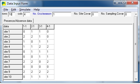
In this example, some detections were uncertain (auditory detection of species) and some detections were certain (eg., visual or both auditory and visual detection of species). Site 1 contains an uncertain detection in survey 3, and site 2 contains an uncertain detecion in surveys 1 and 3, and a certain detection in survey 2.
Alternative False-positive sampling scheme
Instead of having surveys with combined uncertain and certain detections, the sampling scheme may involve two methods of detection, where one method yields certain detections (eg., DNA sample, visual detection), and one method yields uncertain detections (eg., auditory detection). The False-positive model can still be used for these data. The input data would have to be entered such that each survey would occupy two columns in the input file: one column for the uncertain detections and another for the certain detections. Uncertain detections are coded as '1' and certain detections are coded as '2' (as above). The 'trick' needed to make this model work is to fix all of the 'b' parameters (since the probability of a detection being 'certain' is known for all detections). For the columns which correspond to uncertain surveys, the 'b' parameter should be fixed to 0, and the 'b' parameter for columns which correspond to certain detections should be fixed to 1. The probability of false detections, 'p10', should be fixed to 0 for columns which correspond to 'certain' detection surveys.For example, if there are 3 surveys with 'certain' and 'uncertain' detections in each survey, the input detection-history data would contain 6 columns. Columns 1,3,5 would contain uncertain detections in each of the 3 surveys (0=not detected, 1=detected). Columns 2,4,6 would contain certain detections (0=not detected, 2=detected). As far as PRESENCE is concerned, there are 6 surveys, but you will know that there are really only 3 surveys, with two methods per survey.
In the sample below, there are 10 sites and 6 surveys, with the implication that
surveys 1,3,5 are uncertain detections and surveys 2,4,6 are certain
detections.
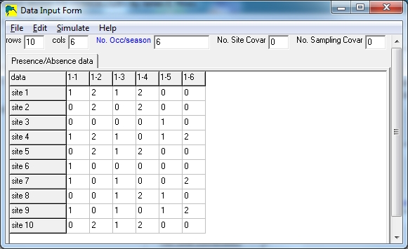
Notice that columns 1,3,5 only contain 0's and 1's, and columns 2,4,6 only
contain 0's and 2's.
When building the model, the detection design matrix will now contain 6 detection probabilities (p11), 6 false-positive probabilites (p10), and 6 'certainty probabilities' (b). Since there cannot be any false-positive detections in surveys 2,4,6, those p10's need to be fixed to zero (p10(2)=0, p10(4)=0, p10(6)=0). Also, since there are no certain detections in surveys 1,3,5, those b's need to be fixed to 0 (b(1)=0, b(3)=0, b(5)=0).
The design matrix and fixed-parameters windows would look like this:
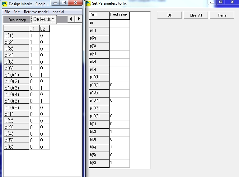
Notice that any parameter which is fixed (right window) contains all zeros for
that row
in the design matrix window (left window). This example design matrix shows a model
where detection probabilities are the same for both methods (p(odd)=p(even)), which
is probably not very realistic. If the methods are drastically different, one would expect
the detection probabilites to be different and model the p's differently.
Staggered-entry model
This model relaxes closure assumption such that a site may locally colonize and go locally extinct once during the surveys (ie., delayed arrival and/or early departure). It is descirbed by Kendall et. al 2013.13. Input data is of the same format as the single-season model.Parameters:
- ψ - probability that the area is occupied by the species,
- bi - probability of species entering between surveys i and i+1, given not entered yet,
- di - probability of species departing between surveys i and i+1, given presence,
- pi - probability of detecting species in survey i, given presence.
Royle/Nichols Occupancy Model for Abundance-induced Heterogeneity
The Royle/Nichols heterogeneity model (Royle and Nichols, 2003) 7 estimates population size from temporally replicated presence/absence data (from point-counts or other types of surveys) at a number of sample sites. This model assumes that heterogeneity in detection probability among sites is due to heterogeneity in abundance (more individuals lead to higher probability of detecting the species at the site). Input data for this model are the presence/absence (1/0) of the species at each survey at each sample site.Parameters estimated under the assumption of a Poisson distribution:
- λ - population density (per site),
- r - probability of detection (per individual of the species)
The species-level probability of detection can be computed using r and λ as:
pi,j = 1 - (1-ri,j)λi
Two-Species Model
The two-species model (MacKenzie et al., 2004) 16 extends the single season model in another way by allowing the computation of occupancy parameters of two species along with conditional probabilities of occupancy when the other species is present or detected.Parameters:
- ψA - probability that the area is occupied by species A,
- ψB - probability that the area is occupied by species B,
- φ - species co-occurance (ψAB/(ψA*ψB)), {ψAB=probability that area is occupied by both species},
- pA - probability of detecting species A, given species B is not present,
- pB - probability of detecting species B, given species A is not present,
- rA - probability of detecting species A, given both are present,
- rB - probability of detecting species B, given both are present,
- λ - species co-detection (rAB/(rA*rB)), {rAB=probability of detecting both species, given both are present},
Input data for this model is in the same form as the single-species, single-season model except that the first half of the detection history records are assumed to be species A, and the second half of the records are assumed to be species B. So, if there are 60 sites, the input would consist of 120 detection history records. Records 1-60 would be the site-detection history records for sites 1-60, species A, and records 61-120 would be the site-detection history records for sites 1-60, species B.
Alternatively, data could be coded without doubling the number of sites. In this case, detections would consist of the following codes:
- 0 = no detection of either species
- 1 = detection of species A only
- 2 = detection of species B only
- 3 = detection of both species
Alternate parameterization
Since two of the parameters in the default parameterization are not probabilities bounded by the interval (0 - 1), numerical problems can arise. (eg., if ψA is zero, φ would be undefined.)An alternate parameterization was developed, using conditional probabilities as parameters, which is more numerically stable. The parameters are:
- ψA - probability that the site is occupied by species A,
- ψBA - probability that the site is occupied by species B, given species A is present
- ψBa - probability that the site is occupied by species B, given species A is not present
- pA - probability of detecting species A, given only species A is present,
- pB - probability of detecting species B, given only species B is present,
- rA - probability of detecting species A, given both are present,
- rBA - probability of detecting species B, given both are present, and species A was detected
- rBa - probability of detecting species B, given both are present, and species A was not detected
Using this parameterization, quantities from the other parametrization can be computed. (eg.,
ψB = ψA*ψBA+(1-ψA)*ψBa
φ = ψA*ψBA/(ψA*ψB)
Two-Species Model with False-positive detections
The Single-season,two-species model (MacKenzie et al., 2004) is extended to allow mis-identification of the species (see Chambert et. al. 201818).Additional parameters:
- ωA - ((oA) in PRESENCE) probability of erroneously detecting species B at a site where only species A is present and species A has also been correctly detected at that site-occasion).
- ωa - ((oa) in PRESENCE) probability of erroneously detecting species B at a site where only species A is present and species A has not been correctly detected at that site-occasion).
- ωB - ((oB) in PRESENCE) probability of erroneously detecting species A at a site where only species B is present and species B has also been correctly detected at that site-occasion).
- ωb - ((ob) in PRESENCE) probability of erroneously detecting species A at a site where only species B is present and species B has not been correctly detected at that site-occasion).
- ηA - ((cA) in PRESENCE) probability that only species A is confirmed at a site that was actually occupied by both species (e.g., only specimens of species A were collected and sent for genetic analyses).
- ηB - ((cB) in PRESENCE) probability that only species B is confirmed at a site that was actually occupied by both species.
Additional data: In order to obtain estimates for this model, additional data are required, in addition to the standard two-species detection data. This additional data consists of a code for each site and survey, indicating which species were confirmed at the site-survey. So, these data should be in the same format as the detection data. For example:
Detection data:                             Confirmation data:
survey  1    2    3    4    5    6          1    2    3    4    5    6

[1,]    2    2    0    2    0    2          0    2    0    2    0    2
[2,]    0    0    0    3    0    2          0    0    0    0    0    0
[3,]    2    0    0    2    0    0          1    0    0    0    0    0
[4,]    3    2    2    2    0    2          3    0    2    0    0    0
Explanation:
- At site, [1,], only species 2 was detected in surveys 1,2,4 and 6. Species 2 was confirmed in surveys 2,4 and 6.
- At site, [2,], both species were detected in survey 4, only species 2 was detected in survey 6. No species were confirmed at any survey.
- At site, [3,], only species 2 was detected in surveys 1 and 4. Species 1 was confirmed in survey 1.
- At site, [4,], both species were detected in survey 1, only species 2 was detected in surveys 2,3,4 and 6. Both species 1 were confirmed in survey 1, only species 2 was confirmed in survey 3.
Input to PRESENCE: The additional confirmation data is entered into PRESENCE as the first "survey covariate", and should be named, "conf".
Single-season-Multi-method Model
The multi-method model (Nichols et al. (2008).
9
)
extends the single
season model by allowing detection probabilities to be different
for different methods of observation. This allows the computation of
an additional parameter, θ which is the probability that
individuals are available for detection at the site, given that they
are present.
Parameters:
- ψ - probability that the area is occupied by the species,
- θx - probability that individuals are available for detection using method x, given presence,
- pxi - probability of detecting species using method x in survey i,
Data input for this model is as follows:
site1  h1,1 h1,2 h1,3... h2,1 h2,2 h2,3...
site2  h1,1 h1,2 h1,3... h2,1 h2,2 h2,3...
site3  h1,1 h1,2 h1,3... h2,1 h2,2 h2,3...
:
:
where hi,j = 1 if detection at site for survey i, method j; hi,j = 0 if no detection
Additionally, the number of methods per survey is specified in the '#meth/srvy' input box, when entering data.
In the sample input below, there are 10 sites, 2 surveys and 2 methods per survey.
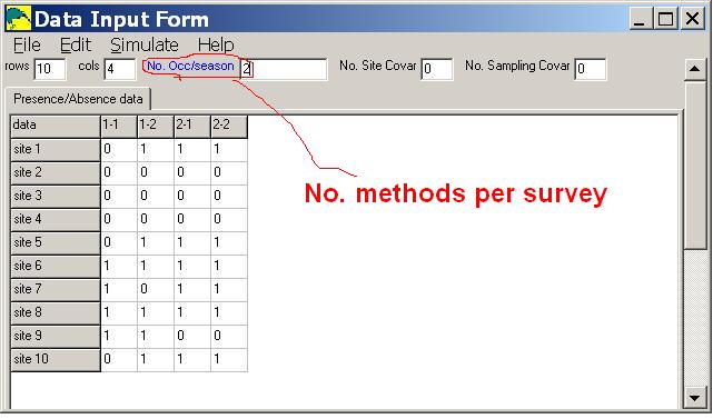
Notice that the column labels (1-1,1-2,2-1,2-2) indicate survey number and method number.
Single-season-Multi-state Model
In the multi-state model (MacKenzie et al., 2009) 5, two kinds of detections are recorded. Detections where only adults observed are recorded as '1' in the data, and detections of known breeding adults (adults seen with young) are recorded as '2' in the data. This allows the computation of an additional parameter, R which is the probability that adults breed, given that they are present.Parameters:
- ψ - probability that the area is occupied by the species,
- R - probability that breeders are present, given the area is occupied by the species,
- p1i - probability of detecting adult non-breeders in survey i,
- p2i - probability of detecting adult breeders in survey i,
- δi - probability of correctly identifying breeders (seeing young with adults) in survey i, given presence,
Input data for this model is in the same form as the single-species, single-season model except that breeding status ('1'=adults only, or '2'=adults and young) is recorded instead of presence ('1').
A more general multi-state model allows for more than just two occupied states. In this case, input consists of:
- 0 = no detection
- 1 = detection of species in state 1 (eg., occupied but no breeding detected)
- 2 = detection of species in state 2 (eg., occupied and breeding detected)
- 3 = detection of species in state 3
- : :
Parameters under this parameterization:
- ψ1 - probability that the area is occupied by the species in state 1,
- ψ2 - probability that the area is occupied by the species in state 2,
- ψ3 - probability that the area is occupied by the species in state 3,
- : - :,
- p11i - probability of observing species in state 1, given it's true state is 1 in survey i,
- p12i - probability of ovserving species in state 1, given it's true state is 2 in survey i,
- p13i - probability of ovserving species in state 1, given it's true state is 3 in survey i,
- : - :
- p21i - probability of observing species in state 2, given it's true state is 1 in survey i,
- p22i - probability of ovserving species in state 2, given it's true state is 2 in survey i,
- p23i - probability of ovserving species in state 2, given it's true state is 3 in survey i,
- : - :
- p31i - probability of observing species in state 3, given it's true state is 1 in survey i,
- p32i - probability of ovserving species in state 3, given it's true state is 2 in survey i,
- p33i - probability of ovserving species in state 3, given it's true state is 3 in survey i,
- : - :
In order for the multi-state model to be identifiable, constraints must be made on the parameters.
- higher-order states must imply presence at lower-order states (eg., breeding implies occupancy, but not vice-versa)
- Due to the 1st constraint, many detection probabilities need to be fixed to zero (eg., p21=0 -> cannot detect breeding if true state = no breeding (1)).