User's Guide for Interactive Program CAPTURE
Eric Rexstad1 and Kenneth Burnham
Colorado Cooperative Fish and Wildlife Research Unit
201 Wagar Building
Colorado State University
Fort Collins CO 80523
1Current address:
Institute of Arctic Biology and
Department of Biology and Wildlife
211 Irving Building
University of Alaska--Fairbanks
Fairbanks, AK 99775-0180
OVERVIEW
This manual describes enhancements to program CAPTURE, previously described in Otis et al. (1978) and White et al. (1982). Program CAPTURE now consists of two executable components: an analytical component that performs abundance and density estimation from information provided by the user (similar to the previous version of CAPTURE), and a new component (2CAPTURE, meaning providing input "to", CAPTURE) allowing easy data entry. Enhancements to the analytical components will be described later. This program can still be run in "batch mode" in the same manner as before; specifying CAPTURE i=<input file> and l=<output file> from the DOS prompt.
Organization of the Users Guide
Because the new version of CAPTURE consists of two distinct programs, they will be described separately. For an overview of the mark-recapture theory under population closure users are directed to Otis et al. (1978); and for general operation of CAPTURE, users are directed to White et al. (1982). For users familiar with the original version of CAPTURE, enhancements to the program will be discussed, and operation of the interactive front-end 2CAPTURE will be described separately.
The interactive component, called 2CAPTURE, represents an interface between the user and program CAPTURE. 2CAPTURE prompts the user for input, examines the users' responses for inconsistencies, formats it in a manner expected by CAPTURE, and calls CAPTURE to perform the desired estimation or simulation. CAPTURE uses an interface familiar to most microcomputer users, popularized by programs such as Lotus 1-2-3; consisting of a top-level menu with pull-down menus and pop-up windows. Interactive help is available for any menu item by pressing the F1 key when the cursor is on a menu item.
Computer System Requirements and Program Dimensions
These programs are designed to run on any IBM-PC compatible computers. Monochrome and color displays are supported. To speed execution, CAPTURE has been compiled (using the Ryan-McFarland FORTRAN compiler) using the capability of a numeric coprocessor (Intel 80x87 chip). If this chip is not
present in the user's computer, CAPTURE will generate an Error 4001 message. Another requirement of the user's computer is adequate memory availability. After loading all memory-resident programs (TSRs, network BIOS, etc.), the user's computer must have approximately 540Kb of available memory to be able to use 2CAPTURE in concert with CAPTURE. Both programs must be resident in memory simultaneously and CAPTURE is approximately 430Kb in size. and 2CAPTURE is 110Kb in size.
The maximum size of analysis problem that can be handled by CAPTURE in this release is 18 capture occasions, 8 nested grids for density estimation, and 1000 animals in simulation experiments. If the user wishes to exceed any of these limitations, CAPTURE must be recompiled after making the requisite
modifications to the file PARMTR.INC. Increasing any of these limits will increase the size of the program, necessitating even greater memory requirements.
Installation and Directory Contents
The distribution disk contains the following files:
Table 1. Contents of distribution disk and brief description of files.
| File |
Description |
| 2CAPTURE.EXE |
Interactive front-end data entry program |
| CAPTURE.EXE |
Abundance and density estimation program |
| LIST.COM |
Shareware file scanner |
| HELPT.TXT |
Narrative for interactive help (Can be modified by user with ASCII word processor) |
| EXAMPLES |
Input file contain examples from Otis et al. (1978) |
| EDWARD.CAP |
Input file used in this guide |
Installation consists of transferring these files to the user's hard disk, preferably to a subdirectory named CAPTURE. By placing this subdirectory in the user's PATH statement, the programs will work as desired when the programs are executed from some other subdirectory. A common situation would then be to keep data files in one subdirectory, and the programs in a separate subdirectory.
2CAPTURE OPERATION
When 2CAPTURE is invoked, the program conducts two internal checks of the machine upon which it is being run. First, 2CAPTURE checks for the presence of a math coprocessor. At present, CAPTURE will not run on machines without a numeric coprocessor. In addition, 2CAPTURE also determines the amount of available memory in the machine after loading 2CAPTURE. If 430Kb of memory is not available after 2CAPTURE has been loaded, 2CAPTURE reports this to inform the user that 2CAPTURE will not be able to invoke CAPTURE, because both programs must reside in memory simultaneously. This does not prevent the user from running 2CAPTURE for the creation of input files, terminating 2CAPTURE prior to invoking CAPTURE, and submitting those input files to CAPTURE in "batch mode."
Top-level 2CAPTURE Menu
After determining the computer system status, 2CAPTURE begins operation by displaying the top-level menu and opening an output window where the file of commands for CAPTURE will be displayed (Fig.l). This window is captioned with the name of the file being created, and the amount of available disk space. These files have the generic name CAPTUR_.INP, where _ is incremented by creation of a new file, e.g. if file CAPTUR4.INP already resides on disk, CAPTUR5.INP will be created.
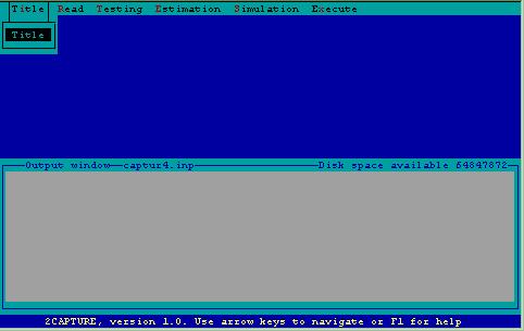
Figure 1. Top-level menu.
The main tasks performed by CAPTURE are listed at the top of the screen and include Title specification, Reading of data, Testing of model fit and assumptions, Estimation of abundance or density, Simulation of data, and Execution of program.
Title menu
The title menu is a very simple menu, consisting of a single choice--namely supplying a title that will appear on each page of printout identifying the run of CAPTURE. After supplying a title, the user is asked to verify this is the desired title. It then appears in the output window enclosed in quotes, as stipulated by CAPTURE.
Read menu
The first step in the estimation of abundance or density is providing data for CAPTURE to analyze. This is accomplished using the read menu (Fig. 2). This menu consists of several subtasks. The task input line being created, to be read later by CAPTURE, is displayed in a window within the output window so the user can see the results of the menu selections.
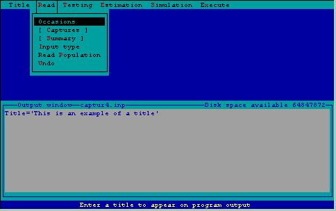
Figure 2. Read menu with associated subtasks.
Read Occasions--Specification of the number of trapping occasions.
Read Captures-- This feature is necessary only if you are reading data from a file and the capture history exceeds the length of records in the file. It is only needed for data types XY reduced and Non XY. This value specifies the number of capture occasions on a single file record.
Read Summary--This provides summary information about the distance moved between captures on output. The average and maximum distances that the animal moved between successive captures, and the average of the maximum distances moved for all animals by the frequency of capture is presented. This can be used to check the reliability of the estimates of density produced by CAPTURE or to construct separate density estimates.
Read Type--There are four methods of entering data to Program CAPTURE. Two methods assume data come from a grid of trapping stations (XY complete and XY reduced). The data entered in these instances are animal ID, and location where trapped on each occasion. If there are no coordinates for trap locations, Non XY input is permitted whereas X-Matrix input presents an animal ID along with a string of 0s and 1s representing occasions on which the animal was captured. Data may either be entered interactively (using 2CAPTURE),or read from a file. If data are read from a file, the user must specify a format statement specifying how data are organized in the records of the file.
A note about format statements. There are 5 types of 'format descriptors' indicating in FORTRAN the way in which data are to be read into a program. These descriptors are T. X, A, I, and F. T and X indicate blank space on an input record which the program is to ignore. The A descriptor indicates character information (words or letters)--the animal ID for CAPTURE is always to be read using the A descriptor. The I descriptor is for integer numbers--this descriptor is never used to read data into CAPTURE. The F descriptor is for real numbers--for example trap location on a grid, or the capture history. As an example, here is a record from the Edward's data set used in the example run at the end of the users guide:
column   1     $    2$        3         4
1234567890123456789012345678901234567890
edwards data  557   11110010001
The animal ID is 557, beginning in column 15, therefore the first part of the format statement for CAPTURE is to skip to column 15, and read the next three characters with the character format descriptor--T15,A3. Following this are three blanks with the next 18 columns representing the capture history for the 18 capture occasions. Therefore the end of the format statement for this data file is 3X,18F1.0. The entire format statement is surrounded by parentheses--(T15,A3,3X,18F1.0). Capitalization and spacing is unimportant. Additional format specifications and the corresponding data can be found in the example input file EXAMPLES on the distribution disk.
Under Read Type are a series of menu choices corresponding to various kinds of input data accepted by CAPTURE.
Read Type XY Reduced--This is the "default" input type. The form of the input is animal ID, occasion on which animal was first caught, x-y coordinates for first capture, occasion of next capture, x-y coordinates of this capture, etc. Therefore, input is only provided when an animal is caught.
Read Type XY Complete- The form of input with XY Complete data is animal ID, x-y coordinates for occasion l, x-y coordinates for occasion 2, etc. If no capture occurred, the coordinates are left blank, or entered as zeroes. XY Complete data types cannot be input interactively. Data must be read from a file, and a format statement must be specified. Interactive input of data containing x-y coordinates can more easily be accomplished using the XY Reduced data type.
Read Type Non-XY--If trap coordinates are to be ignored, density cannot be estimated by CAPTURE, but abundance may be estimated. The form of Non-XY input is animal ID, first capture occasion, second capture occasion, etc. Data must be read from a file, and a format statement must be specified. Interactive input of data of this form can more easily be accomplished using the X-Matrix data type.
Read Type X-Matrix-- If trap coordinates are to be ignored, density cannot be estimated by CAPTURE, but abundance may be estimated. The form of X-Matrix input is animal ID, and a string of 0s and 1s (one such character for each capture occasion) signifying whether the individual was captured (1) or not (0) on each occasion.
Read Population--If complete capture history information is not available, the user may enter sufficient or minimal sufficient statistics to compute an estimate of population size. Each estimator has specific minimal
sufficient statistics required to compute a population estimate. Model selection is, of course, not performed when the user specifies the estimator to use.
Under this subtask there are a number of estimators that have been programmed into CAPTURE. In all cases, the number of capture occasions (t) is required, along with other statistics summarized from the data, as described below. Note the estimator for Mth must have the raw data to obtain an estimate, therefore there is no "Read Population" choice for it.
Read Population Null - Minimal sufficient statistics for the estimator under M0 are the total captures (n.), and total unique individuals captured (Mt+1)
Read Population Jackknife--Minimal sufficient statistics for the estimator under Mh are the number of individuals captured one time (f1), twice (f2), three times (f3), etc.
Read Population Removal--Minimal sufficient statistics for the estimator under Mbh are the number of unmarked individuals captured on each occasion (ui)
Read Population Darroch--Minimal sufficient statistics for the estimator under Mt are total unique individuals captured (Mt+1), and number of individuals captured on each occasion (ni). Of course, each ni must be less than or equal to Mt+1
Read Population Zippin--Sufficient statistics for the estimator under Mb are the number of unmarked individuals captured on each occasion(ui).
Read Population Chao Mt--Minimal sufficient statistics for the estimator under Mt are the number of individuals captured one time (f1), twice (f2), three times (f3), etc.
Read Population Chao Mh--Minimal sufficient statistics for the estimator under Mh are the number of individuals captured one time (f1), twice (f2), three times (f3), etc., and number of individuals captured only on occasion 1 (z1), only on occasion 2 (z2), only on occasion 3 (z3), etc. As a check, performed by 2CAPTURE, the sum of the (z1), must be equal to f1
Read Population Burnham Mtb-- Minimal sufficient statistics for the estimator under Mtb are the number of individuals captured on each occasion (ni), ant number of marked individuals in the
population immediately prior to each occasion (Mi-1), including Mt+1
Read Undo--This command is used if the user misspecifies any information on the TASK READ CAPTURES record, e.g. if Occasions is misspecified or if input data type is entered incorrectly. This command will not allow correction of errors committed during the actual input of capture history data.
Testing menu
An important part of population estimation is selecting the appropriate model to perform estimation. Selection of the appropriate model is dependent upon testing the assumptions of the models. These tests, along with a test for population closure are constructed from the testing menu (Fig. 3).
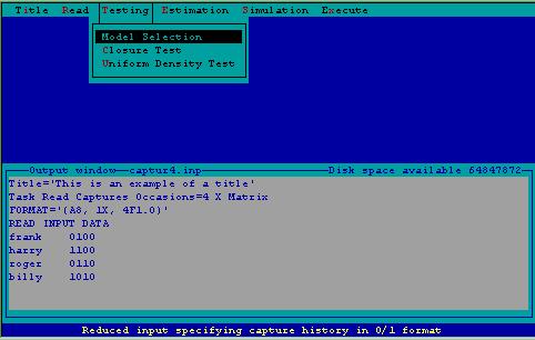
Figure 3. Testing menu.
Model Selection--This invokes a model selection algorithm described in Otis et al. (1978:57-61) examining the data set through a series of tests looking for time, behavior, and heterogeneity effects. A discriminant function procedure selects the most appropriate model for the data based on these tests. Test results are only printed when the model selection option is chosen. It is recommended this task be performed. The "Appropriate" estimator (chosen by the model selection algorithm) can only be used when model selection is performed.
If the user wishes, the occasions tested need not match the number of occasions recorded. In this case, using a hyphen '-' between two numbers indicates only occasions specified will be analyzed (e.g., 1-5). Commas may also be used to separate sequences of numbers so that 1-5,9-10,12 means the series of occasions 1,2,3,4,5,9,10, and 12 will be analyzed.
Closure Test--The estimators used in this program assume the population is closed. meaning the composition and size of the population remains constant for the duration of the study. This test attempts to determine statistically if this assumption is met. The test has poor power and is seldom capable of properly rejecting the null hypothesis of closure. This test is described in Otis et al. (1978:66).
If the user wishes, the occasions tested need not match the number of occasions recorded. In this case, using a hyphen '-' between two numbers indicates only occasions specified will be analyzed (e.g., 1-5). Commas may also be used to separate sequences of numbers so that 1-5,9-10,12 means the series 1,2,3,4,5,9,10, and 12 will be analyzed.
Uniform Density Test--If XY-complete or XY-reduced input is provided, a statistical test to determine uniformity of distribution of individuals in the trapping grid is performed.
If the user wishes, the occasions tested need not match the number of occasions recorded. In this case, using a hyphen '-' between two numbers indicates only occasions specified will be analyzed (e.g., 1-5). Commas
may also be used to separate sequences of numbers so that 1-5,9-10,12 means the series 1,2,3,4,5,9,10, and 12 will be analyzed.
Estimation menu
After providing data, and optionally specifying tests to be performed, the actual estimation (either abundance or density) can be done. In this step, the estimators to be used are specified. First, the issue of abundance estimation.
Abundance Estimation
Estimate Population--CAPTURE can produce estimates of either population abundance or population density. Estimation of abundance produces an estimate of the number of individuals in the population at risk of capture. Point estimates along with 95% confidence intervals are produced.
Estimate Population Occasions--If the user wishes, the occasions used for population estimation need not match the number of occasions recorded. In this case, using a hyphen '-' between two numbers indicates only occasions specified will be analyzed (e.g., 1-5). Commas may also be used to separate sequences of numbers so that 1-5,9-10,12 means the series 1,2,3,4,5,9,10, and
12 will be analyzed.
Estimate Population Estimators--Ten different estimators of population size can be used in program CAPTURE. These include 2 estimators for the model of time effects (Darroch and Chao Mt.), three for the model of heterogeneity effects (Jackknife and Chao Mh); single estimators for models of behavior effect (Zippin [Mb]), time and heterogeneity effects (Chao Mth), time and behavior effects (Burnham Mtb), behavior and heterogeneity effects (Removal
and Pollock and Otto's estimator)[Mbh], and the null model of no time, behavior or heterogeneity effects [Mo]. There is currently no estimator for model Mtbh. All estimators can be invoked by selecting ALL, and the most appropriate mode) can be chosen using APPROPRIATE (if task model selection has been invoked). Multiple estimators can be selected for a single data set. See description of the various estimators below.
Estimate Population Undo--If OCCASIONS parameter or estimators are inappropriately specified, (this can be detected by examining the Estimate Population window), selecting Undo will obliterate this task card without adding it to the output file. After undoing the incorrect task, Occasions or Estimators can be specified correctly.
Density estimation
Estimate Density--This program can produce estimates of either population abundance or population density. Estimation of abundance produces an estimate of the number of individuals in the population at risk of capture. Point estimates along with 95% confidence intervals are produced when the procedure works. The nested grid approach is known to fail frequently; other methods of density estimation can be employed using N produced by CAPTURE.
Density is estimated using the nested-grid approach from data derived from a lattice of equally-spaced trap locations. Grid definitions must be specified. Each grid must specify values for two parameters: X= and Y= determine the range of x- and y- coordinates for the grid. For example, X=5-9 Y=3,8 specified a 5 by 6 grid with lower left corner at (5,3). Either a hyphen or comma may be used to separate the values. See Otis et al. (1978:67-72).
Estimate Density Intervals--The distance between traps must be specified for proper density estimation. For example, if traps are 15 meters apart, 15 is specified. The units are not required, but conversion from linear distance to area is performed by the program (see Conversion).
Estimate Density Conversion-- Conversion from linear distance to area. If distance between traps is measured in meters, a conversion factor of 1 results in animals per meter. The default conversion factor of 10000 assumes distance between traps is measured in meters and resulting density is expressed in animals per hectare. If distance between traps is measured in feet, and density is to be expressed in animals per acre, the conversion factor is 43560.
Estimate Density Occasions- If the user wishes, the occasions used for density estimation need not match the number of occasions recorded. In this case, using a hyphen '-' between two numbers indicates only occasions specified will be analyzed (e.g., 1-5). Commas may also be used to separate sequences of numbers so that 1-5,9-10,12 means the series 1,2,3,4,5,9,10, and 12 will be analyzed.
Estimate Density Estimators--Seven different estimators of population density can be used in program CAPTURE. These include estimators for the model of time effects (Darroch), the model of heterogeneity effects (Jackknife) the model of behavior effect (Zippin), time and heterogeneity effects (Chao Mth), time and behavior effects (Burnham Mtb), behavior and heterogeneity effects (Removal), and the null model of no time. behavior or heterogeneity effects. There is no estimator for model Mtbh. All estimators can be invoked by selecting ALL, and the most appropriate model can be chosen using APPROPRIATE (if task model selection has been invoked). Multiple estimators can be selected for a single data set. See description of estimators below.
Estimate Density Undo--If Interval, Conversion, or Estimators are inappropriately specified, selecting Undo will obliterate this task card without adding it to the output file. After undoing the incorrect task, Interval, Conversion, or Estimators can be specified correctly.
Estimators menu
For both abundance and density estimation, a series of estimators have been developed to model capture probabilities. These estimators can be selected by the user, or chosen by the model selection algorithm described in the testing section. An example of the estimator selection menu associated with abundance estimation is displayed in Fig. 4.
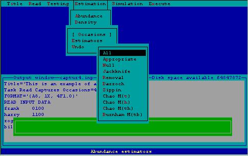
Figure 4. Estimator menu associated with abundance estimation.
Estimator All-- All estimators are used to estimate abundance or density from the data given.
Estimator Appropriate--If Task Model Selection has been specified, the model selection algorithm will select the model most appropriate for the given data set, and the estimation of abundance (or density) will be performed under this model.
Estimator Null--The simplest of all models, M0 assumes all members of the population are equally at risk of capture on every trapping occasion. Parameters estimated are population size and a single probability of capture. See Otis et al. (1978:21-24).
Estimator Jackknife--This is the estimator for Mh which assumes capture probabilities vary by individual animal. Parameters estimated are population size and probabilities of capture for each individual. Of course, estimation of unique capture probabilities for each individual is impossible, rather the probability distribution is estimated. See Otis et al. (1978:33-37).
Estimator Removal--This is the estimator for Mbh which assumes capture probabilities vary by individual animal and by behavioral response to capture. Parameters of this model would include population size, and two probabilities of capture for each individual in the population. Obviously this number of parameters cannot be estimated from capture-recapture data. Instead, only the number of unmarked individuals captured on each occasion is used in estimation. At least three occasions are necessary for goodness-of-fit testing. See Otis et al. (1978:40-50).
Estimator Darroch--This is the estimator for Mt which assumes capture probabilities vary with time. Parameters estimated are population size and probability of capture for each occasion. When there are only two occasion, this reduces to the familiar Lincoln-Petersen Index. See Otis et al. (1978:25-28).
Estimator Zippin--This is the estimator for Mb which assumes capture probabilities vary by behavioral response to capture. Parameters estimated are population size, probability of capture of an unmarked animal on any trapping occasion, and the recapture probability of any animal captured at least once. See Otis et al. (1978:28-32).
Estimator Chao Mt--This is the estimator for Mtwhich assumes capture probabilities vary with time. Parameters estimated are population size and probability of capture for each occasion, as described in Chao (1989). When probabilities of capture are small, this estimator performs well.
Estimator Chao Mh--This is the estimator for Mh which assumes capture probabilities vary by individual animal. Parameters estimated are population size and probabilities of capture for each individual. As described in Chao (1988), when probabilities of capture are small, this estimator is less biased than the jackknife estimator.
Estimator ChaoMth--This is the estimator for Mth which assumes capture probabilities vary with time and by individual. Parameters estimated are population size, and average capture probabilities for each occasion.
Estimator Burnham Mtb--This is the estimator for Mtb which assumes capture probabilities vary with time and with behavioral effects (trap happiness trap shyness). The model used is that recapture probability is some function of initial capture probability [c = P1/theta]. Parameters estimated are population size, initial capture probabilities, and # A variance-covariance matrix of parameter estimates is also produced. along with a goodness-of-fit test.
Simulation menu
If performance of estimators, or if questions of study design are of interest, data may be simulated by program CAPTURE. Output can be examined to determine effects of not meeting assumptions of various estimators, etc. Numerous options are available to allow the user great flexibility in conducting the simulation experiment. These options are displayed in Fig. 5, and discussed below. The TASK SIMULATE "card" is constructed in a window displayed inside the output window so the user can see the results of selection of various menu items.
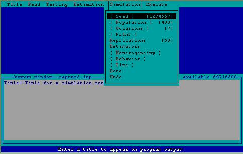
Figure 5. Simulation menu.
Simulation Seed--This is a random integer used as a starting value to generate random numbers between zero and one. The default value is 1234567. If you wish to repeat a set of simulations, the seed must be the same for each repeated run.
Simulation Population Size--This specifies the size of the population to be simulated. The default value is 400, a maximum population of 1000 individuals is currently allowed.
Simulation Occasions--This specifies the number of trapping occasions to be simulated. The default number is 7, with a maximum of 31 allowed.
Simulation Print--This is a switch that results in a complete printed output for each replicate. If the user is interested in results of the various tests associated with model selection, this will cause the tests to be printed. Beware that the amount of output generated will be very large when the number of replicates is large. Do not use this switch when more than 10 replicates are specified. If "Print" is not specified, only the table of summary statistics for the simulations will be printed.
Simulation Replicates--This specifies the number of simulation trials to be conducted. The default value is 50, with no maximum. The number of replications will determine the confidence in the output, i.e., the precision of the estimates.
Simulation Estimators--This forces a particular estimator to be used for the simulated data. No more than one estimator may be specified for a simulation experiment. See Estimators section above for a description of various estimators available. If multiple estimators are of interest, multiple simulation experiments must be performed. If no estimator is specified, the model selection algorithm will pick the estimator most appropriate for the simulated data set.
Simulation Heterogeneity--This specifies the probabilities of capture of individuals in the simulated population will be heterogeneous. The standard way of accomplishing this is to comprise the population of homogeneous subpopulations. The user specifies the number of individuals in the subpopulation, and their associated probability of capture until all members of the population have been accounted for. Capture probabilities may also be specified as beta distributions. This cannot be accomplished with 2CAPTURE, but can be constructed in the input file submitted to CAPTURE in batch mode. Specifying beta(alpha, beta, lbnd, ubnd) indicates a beta distribution with parameters alpha and beta and generates capture probabilities in the range (lbnd, ubnd). Additionally, 'time varying' on the simulate card indicates that heterogeneity and behavior probabilities generated from a beta distribution will change on each capture occasion.
Simulation Behavior--This specifies the probabilities of capture of individuals in the simulated population will be capture-history specific. The standard way of accomplishing this is to comprise the population of homogeneous subpopulations. The user specifies the number of individuals in the subpopulation, and their associated recapture probability (as a multiplier) until all members of the population have been accounted for. Capture probabilities may also be specified as beta distributions. This cannot be accomplished with 2CAPTURE, but can be constructed in the input file submitted to CAPTURE in batch mode. Specifying beta(alpha, beta, lbnd, ubnd) indicates a beta distribution with parameters alpha and beta and generates capture probabilities in the range (lbnd, ubnd). Additionally, 'time varying' on the simulate card indicates that heterogeneity and behavior probabilities generated from a beta distribution will change on each capture occasion.
Simulation Time--This specifies the probabilities of capture of individuals in the simulated population will be time specific. The user specifies the probability of capture for each capture occasion to be simulated. Capture probabilities may also be specified as beta distributions. This cannot be accomplished with 2CAPTURE, but can be constructed in the input file submitted to CAPTURE in batch mode. Specifying beta(alpha, beta, lbnd, ubnd) indicates a beta distribution with parameters alpha and beta and generates capture probabilities in the range (Ibnd, ubnd). Additionally, 'animal varying' on the simulate card indicates that time-specific probabilities generated from a beta distribution will vary by animal on each capture occasion.
Simulation Done--After all parameters for the simulation experiment have been specified, the Task Simulate must be designated as complete. Selecting this option will close the Task Simulate window and place the Information into the output file window.
Simulation Undo--If any parameter, with the exception of the heterogeneity, behavior, and time structures, associated with Task Simulate are misspecified, selecting this option will close the Task Simulate window
without placing the information into the output file window. The user may then begin again to specify the structure of the Task Simulate.
Execution menu
When all input has been specified for program CAPTURE, the program is invoked, output can be examined, temporary and permanent return to the operating system is accomplished here. These options are shown in Fig. 6.
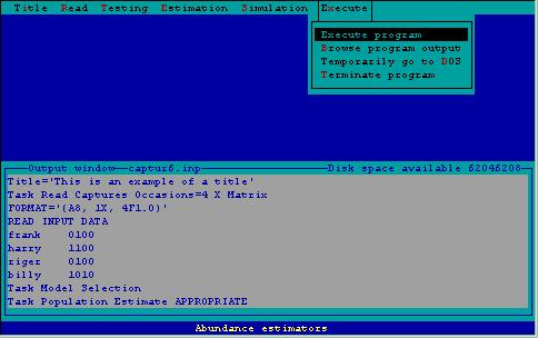
Figure 6. Execution menu.
Execute Program Execution--AFter specifying statements needed by program CAPTURE, this step is invoked. Statements in the output window are sent to program CAPTURE, and abundance/density estimation or simulation is performed. An output file is created by program CAPTURE, as specified on the bottom status line. After program execution is completed, control returns to 2CAPTURE for subsequent specification of additional input.
Execute Browse Output--When data have been analyzed by program CAPTURE, the results are sent to an output file. This file can be examined by invoking this command. A shareware program LIST is called to examine the output file just created. Using PgUp, PgDown allow the user to examine the output prior to printing. Pressing ? will provide a full list of commands available with LIST. The F command is particularly useful; it 'finds' a text string in the file. Searching for the string 'estimate' is a quick way of identifying point estimates produced by various estimators. Pressing either X or ESC terminates LIST and returns control to 2CAPTURE.
Execute Shell to Operating System--If the user wishes to temporarily leave 2CAPTURE and return to the operating system, invoke this command. For example, if the user wishes to rename an output file, or print the output file, this can be done by temporarily returning to the operating system, performing the necessary tasks, and returning to 2CAPTURE. Return to 2CAPTURE is accomplished by typing 'EXIT'.
Execute Terminate--Invoke this command when all data have been analyzed and permanent return to the operating system is desired.
NEW FEATURES ADDED TO PROGRAM CAPTURE
Users familiar with the original version of CAPTURE, and who choose not to use interactive 2CAPTURE, will need to know about several program revisions. These revisions are shown in Table 2.
Table 2. Revisions to estimators in program CAPTURE
| Model |
Revisions |
| M0 |
New configence interval estimate |
| Mt |
New configence interval estimate |
| Competing estimator (Chao's Mt) |
| Mb |
New confidence interval estimate |
| Mh |
New standard error estimate |
| New confidence interval estimate |
| Competing estimator (Chao's Mh) |
| Mbh |
New confidence interval estimate |
| Competing estimator (Pollock and Otto's Mbh) |
| Mth |
New estimator |
| Mtb |
New estimator |
| Mtbh |
No revisions, no estimator |
Output generated by CAPTURE is now contained within 80 columns, for ease of printing and viewing on computer screens. Output has also been streamlined with notation definitions and some intermediate results suppressed unless the word "verbose" appears on the command line when CAPTURE is run in batch-mode. Batch mode is invoked from DOS by executing C> CAPTURE i=<input file name>I=<output file name>
The most sweeping of these revisions is the inclusion of new estimators for Mth and M'`, as well as competing estimators for Mh and Mt. In order to access these estimation routines, the user must know the key words recognized by CAPTURE to invoke each of these estimators, shown in Table 3.
Table 3. Estimators and their associated key words, new estimators are shown in boldface
| Model |
Estimator Key word |
| M0 |
Null |
| Mt |
Darroch |
| Mt-Chao |
| Mh |
Jackknife |
| Mh-Chao |
| Mb |
Zippin |
| Mbh |
Removal |
| Mth |
Mth-Chao |
| Mtb |
Mtb-Burnham |
Note that only the first four characters of the key words are necessary to identify the estimator to CAPTURE and capitalization is optional. Note also when the Removal estimator is requested the estimator of Pollock and Otto (1983) is also printed, but is not used for subsequent calculations as when simulation is performed.
New estimators and their sufficient statistics
For all estimators described, the number of capture occasions (t) is required, along with the statistics described below.
Chao's Mt--Data necessary to estimate abundance with this estimator are the number of individuals captured i times where i=1, 2, ..., t. These are the capture frequencies fit See Chao (1989) for a complete description of this estimator.
Chao's Mh--Data necessary to estimate abundance with this estimator are the number of individuals captured i times where i=1, 2, ..., t. These are the capture frequencies (f1), In addition, the number of individuals captured only once on occasions 1 through t are needed. Chao (1989) refers to these statistics as (zi), where (zi), is the number of individuals captured only on occasion i. See Chao (1989) for a complete description of this estimator.
Chao's Mth--There are no sufficient statistics for Mth because the entire capture history array 1s necessary to calculate this estimator. See Chao et al. (in press) for a complete description of this estimator.
Burnham's Mtb--Data necessary to estimate abundance with this estimator are the number of individuals captured on each occasion (ni), and number of marked individuals in the population immediately prior to each occasion (Mi-1).
Confidence interval calculation for all estimators
Problems have been know to exist with the confidence interval estimation of N. Confidence interval calculations for all estimators have been revamped to attempt to remedy some of these problems.
One of the problems is that lower bounds of the confidence interval fall below the number of distinct individuals captured (Mt+1), an absurdity because the number of individuals in the population is known to be at least as large as Mt+1 Previous remedies to this problem have been to truncate the confidence interval at Mt+1, this is an undesirable ad hoc approach with no basis in statistical theory.
Another difficulty associated with confidence interval estimation on N is the non-normal distribution of N. Asymptotic normality is an underlying assumption of classical methods of calculating confidence intervals using +- 1.96.SE(N). The non-normality of the distribution of N leads to poor coverage of the true population size by the confidence interval.
An approach described by Burnham et al. (1987:211-213) and applied by Chao (1989:429) has been implemented for all estimators in CAPTURE. It is based on the assumption that the number of individuals in the population not captured (N - Mt+1) is log-normally distributed. Under this assumption, the confidence interval bounds are calculated as
where f0 is the number of individuals not captured (N - Mt+1) and
From these calculations, it is clear that the lower bound of the confidence interval cannot be less than Mt+1. The upper bound also tends to be larger than upper bounds calculated in the classic fashion, leading to better confidence interval coverage.
Profile likelihood intervals
An alternative approach to calculating confidence intervals is based on the asymptotic c2 distribution of the generalized likelihood ratio test (Venzon and Moolgavkar 1988; Hudson 1971). The maximum likelihood estimate of population size, N is at the point where the likelihood is maximized, call this likelihood value max. At some point below that maximum, 1.92 units below from the properties of the c2 distribution, the values of the parameter N where the likelihood takes on the value max-1.92 are bounds of the profile likelihood interval. Brief mention of profile likelihood intervals is made by Otis et al. (1978:133-135) in Appendix O.
The null estimator (m0) Darroch's estimator (Mt), the Zippin estimator (Mb) the generalized removal estimator (Mbh), and Burnham's Mtb estimator all have explicit likelihoods. For each of these estimators, the calculation of the profile likelihood interval is performed and reported by CAPTURE. Cursory examination of these intervals have shown them to be quite close to the log-based confidence intervals described above. However, the log-based confidence intervals are the intervals computed when simulation experiments are conducted using CAPTURE; profile intervals are only reported when the Print option is used with Task Simulate.
Variance calculation for Jackknife estimator
The calculation of var(NJ) described in Otis et al. (1978:109) has been known from simulation experiments to be biased low (Otis et al. 1978:34-35) leading to poor coverage. A new method of calculating var(NJ)
has been incorporated into this release of CAPTURE.
A number of estimators (n(est) = min(5, t)) are computed under the jackknife method used for Mh. Based on n(est)-1 tests between successive estimators, one estimator is chosen for a given data set, say NJi. Previously in CAPTURE the conditional variance of the selected NJi was then used. Experience has shown this conditional procedure gives, on average, variances that are too small. The (ni), unconditional variance of NJ is needed, var(NJ). Var (NJ) is calculated as N
where
probability of the ith estimator being the estimator of choice (pi) is determined by the c2 test between successive estimators; more precisely, pi depends on the power of that test (1-bi) For the case of n(est) = 5, the pi are
p1=b1
p2=(1-b1)b2
p3=(1-b1)(1-b2)b3
p4=(1-b1)(1-b2)(1-b3)b4
p5=(1-b1)(1-b2)(1-b3)(1-b4)
When n(est) = k is less than 5, the last pk is just 1-(p1+...+pk-1). The actual test statistics are used as a
basis to estimate the b. Estimators for which there is good power of the c2 test contribute highly to the expected value of NJ, and consequently contribute highly to the calculation of var(NJ). Cursory simulation studies demonstrate that calculation of var(NJ) in this manner, coupled with the modified confidence interval estimation described above, result in much improved coverage levels for the jackknife estimator.
Summary of simulation experiments
A few modifications have been made to the summary of simulation experiments. Obviously, because estimates are now available for Mth and Mtb, numerical values are now printed in the summary table when either those estimators are chosen by the user, or selected by the model selection algorithm. Behavior of Chao's Mt (Chao 1989) and Mh (Chao 1988) can also be investigated via simulation if the user explicitly chooses those estimators; they are not selected by the model selection algorithm. Therefore the values in the summary tables for Mt and Mh may represent different estimators dependent upon the input provided by the user. Pollock and Otto's (1983) Mbhestimator can be explicitly simulated, but when the model selection algorithm is used, the generalized removal estimator described in Otis et al. (1978:112-113) is employed. Users who wish to employ profile likelihood intervals rather than the log-based confidence intervals may investigate the performance of these intervals via simulation placing the keyword "PROFILE" on the Task Simulate card.
Overall averages of point estimates, standard deviations, and confidence interval coverage for all models are now provided. As an example, Table 4 below demonstrates the results from an experiment with 100 replications where capture probabilities are simulated under Mtbh and the model election algorithm selects the most appropriate model for each replication.
Table 4. Example output from simulation experiment with N=100, 100 replicates of Mtbh.
| Model Selection Results |
Point Estimates |
| Model |
Times
Selected |
Percent
Selected |
Failures |
Average
Estimate |
Standard
Deviation |
Lower
Confidence
Bound |
Upper
Confidence
Bound |
| Mo |
59 |
59.00 |
0 |
54.71 |
11.577 |
51.76 |
57.67 |
| Mh |
9 |
9.00 |
0 |
72.48 |
14.987 |
60.96 |
84.00 |
| Mb |
0 |
0.00 |
0 |
0.00 |
0.000 |
0.00 |
0.00 |
| Mbh |
0 |
0.00 |
0 |
0.00 |
0.000 |
0.00 |
0.00 |
| Mt |
14 |
14.00 |
0 |
56.36 |
9.834 |
50.68 |
62.03 |
| Mth |
9 |
9.00 |
0 |
56.23 |
12.047 |
46.97 |
65.49 |
| Mtb |
0 |
0.00 |
0 |
0.00 |
0.000 |
0.00 |
0.00 |
| Mtbh |
9 |
9.00 |
0 |
0.00 |
0.000 |
0.00 |
0.00 |
| Total |
91 |
|
|
56.87 |
12.678 |
54.27 |
59.48 |
Interval Estimate Lengths |
| Model |
Coverage |
Percent
Coverage |
Failures |
Average
Interval
Length |
Standard
Deviation |
Lower
Confidence
Bound |
Upper
Confidence
Bound |
| Mo |
15 |
25.42 |
0 |
46.61 |
22.697 |
40.82 |
52.40 |
| Mh |
6 |
66.67 |
0 |
46.43 |
8.409 |
39.96 |
52.89 |
| Mb |
0 |
0.00 |
0 |
0.00 |
0.000 |
0.00 |
0.00 |
| Mbh |
0 |
0.00 |
0 |
0.00 |
0.000 |
0.00 |
0.00 |
| Mt |
3 |
21.43 |
0 |
42.67 |
15.724 |
33.59 |
51.74 |
| Mth |
5 |
55.56 |
0 |
63.52 |
27.258 |
42.57 |
84.47 |
| Mtb |
0 |
0.00 |
0 |
0.00 |
0.000 |
0.00 |
0.00 |
| Mtbh |
0 |
0.00 |
0 |
0.00 |
0.000 |
0.00 |
0.00 |
| Total |
29 |
31.87 |
|
|
|
|
|
Note that the total number of experiments printed at the bottom of the point estimate table disregards the number of times Mtbh is selected. If there had been any estimator failures, these would have also been subtracted. Averages and overall standard deviation and confidence intervals are based on this sample size (91 in this case). Additionally, total percent coverage in the second table is calculated on the basis of n=91; therefore 29 of 91 replicates cover the true population size of 100, for a total coverage level of 31.87%.
SAMPLE PROGRAM RUN AND OUTPUT ANNOTATION
An interesting example of the operation of 2CAPTURE and CAPTURE is the data collected by Edwards and Eberhardt (1967) from a penned population of 135 wild cottontails Sylvilagus floridanus. These data combine the reality of a field study with the ability to contrast behavior of estimators with a known population size.
The data were stored in X-matrix format in a file called EDWARD.CAP. Steps used to prepare these data with 2CAPTURE for analysis with CAPTURE are shown in Figures 7-9.
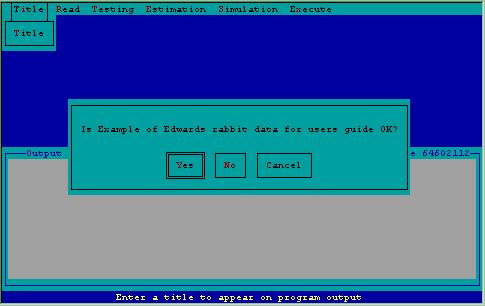
Figure 7. Specification of title for analysis of Edward's data inquiring about certainty of title.
Figure 8 demonstrates specification to 2CAPTURE to read the actual capture histories from a file, called EDWARD.CAP. 2CAPTURE looks in the current subdirectory for a file with the name specified; if it fails to find the file, an error message will flash on the screen with a request to respecify the filename.
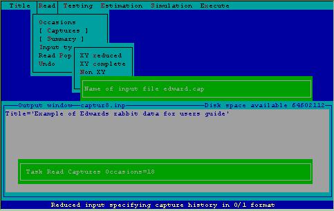
Figure 8. Specifying a file from which to read capture histories.
Giving a format statement with which CAPTURE reads the capture histories is the step that causes users great consternation. 2CAPTURE offers the user the opportunity to scrutinize the file that will be read prior to specifying the format. In the case of EDWARD.CAP, the first 14 columns of each record contain indentifying information about the data set. The next 3 columns contain the animal identification number, which must be read by CAPTURE. Following 3 blanks, the 18 capture occasions (with 0 for no capture, 1 for a capture) appear on each record. The appropriate format for reading these data as entered via 2CAPTURE is shown in Fig. 9.

Figure 9. Specifying an input format for file containing capture histories.
The abbreviated output generated by CAPTURE from these data is shown by clicking here Some notes regarding the output are interspersed in program output.
These results can be contrasted with results shown on pages 84-86 of Otis et al. (1978). It is interesting to note that of the 10 estimators now calculated by CAPTURE, 5 confidence intervals cover the true population size of 135, and 5 confidence intervals do not cover the true value. Of the 5 intervals that cover the true value, 4 are for new estimators added in this new release of CAPTURE.
FUTURE WORK
Incorporation of profile likelihoods into the simulation procedure has not yet been performed. We are confident of the estimators with the possible exception of Mtb. The model selection algorithm is in need of extensive work, and some of the tests upon which model selection is based may be enhanced. Users receiving this version of CAPTURE will receive future revisions of the code.
ACKNOWLEDGEMENTS
Funding for this work was provided by the U.S. Fish and Wildlife Service Region 6 Enhancement Program through the Rocky Mountain Arsenal. Thanks to Gary White and David Anderson for advice and comments on computer coding and this users guide.
LITERATURE CITED
Chao, A. 1988. Estimating animal abundance with capture frequency data. J. Wildl. Manage. 52:29 300.
. 1989 Estimating population size for sparse data in capture-recapture experiments. Biometrics 45:427-438.
________ S. M. Lee, and S. L. Jeng. In press. Estimation population size for capture-recapture data when capture probabilities vary by time and individual animal. Biometrics.
Hudson, D. J. 1971. Interval estimation from the likelihood function. J. R. Stat. Soc. B 33:256-262.
Otis, D., K. P. Burnham, G. C. White, and D. R. Anderson. 1978. Statistical inference from capture data on closed animal populations. Wildl. Monogr. 62:1-135.
Pollock, K. H., and M. C. Otto. 1983. Robust estimation of population size in closed animal populations from capture-recapture experiments. Biometrics 39:1035-1049.
Venzon, D. J., and S. H. Moolgavkar. 1988. A method for computing profile-likelihood-based confidence intervals. Appl. Statist. 37:87-94.
White, G. C., D. R. Anderson, K. P. Burnham, and D. L. Otis. 1982. Capture-recapture and removal methods for sampling closed populations. Los Alamos Nat. Lab. Publ. LA-8787-NERP. 235pp.