Applied hierarchical modeling in Ecology

by Marc Kéry & Andy Royle

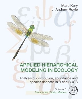
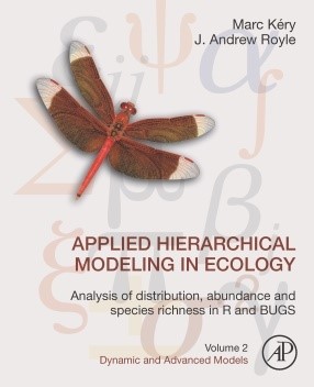
This is the permanent book web site of the Applied hierarchical modeling (AHM) project. It comprises two volumes of a book with the same name and the R package AHMbook which can be downloaded from CRAN; our BIG thanks for this go to Mike Meredith!

We plan to publish the solutions to some or all the exercises in AHM volume 1, but this will likely have to wait until AHM volume 2 is written (which will be the end of 2019).

For a more dynamical (i.e., more frequently updated) AHM page, see our Google page here: https://sites.google.com/site/appliedhierarchicalmodeling/home

Get your copy of the book from Amazon:
http://www.amazon.com/Applied-Hierarchical-Modeling-Ecology-distribution/dp/0128013788/ref=sr

Overview of chapters in volumes 1 and 2 of AHM:

AHM Volume 1: Prelude and static models

Preface

Part 1: Prelude

Distribution, abundance and species richness in ecology
What are hierarchical models and how do we analyze them?
Linear models, generalized linear models (GLMs), and random-effects: the components of hierarchical models
Introduction to data simulation
The Bayesian modeling software BUGS and JAGS

Part 2: Models for static systems

Modeling abundance using binomial N-mixture models
Modeling abundance using multinomial N-mixture models
Modeling abundance using hierarchical distance sampling
Advanced hierarchical distance sampling
Modeling distribution and occurrence using site-occupancy models
Community models

AHM Volume 2: Dynamic and Advanced models

Part 3: Models for dynamic systems

Poisson Generalized Linear Mixed Models (GLMMs) and related models
Modeling population dynamics with replicate counts within a season
Modeling population dynamics with distance sampling data
Hierarchical models of survival
Modeling species distribution and range dynamics using dynamic occupancy models
Modeling metacommunity dynamics using dynamic community models

Part 4: Advanced models

Multi-state occupancy models
Modeling false-positives
Models for species interactions
Spatial models I
Spatial models II
Combination approaches / Integrated models
Spatial distance sampling and spatial capture-recapture

Conclusions

The new AHMbook R package

To install the AHMbook R package, you need R version 3.3.0 or later. Thanks to the efforts of Mike Meredith, AHMbook is now a genuine R package, so you can download it from CRAN in the usual way, e.g., by typing in your R console

install.packages("AHMbook")

The new R and JAGS code

Mike Meredith has translated the published book code so that it is compatible with the new AHMbook R package. You can download it here:

R_BUGS_code_AHM_Vol_1_20170519.R

List of detected errors:

link [https://sites.google.com/site/appliedhierarchicalmodeling/errata]

For backwards compatibility with the printed book, we provide the original four extra data files and the original R/BUGS code here.

Four AHM extra data files

We used to supply four additional data files that are used in AHM1: the Swiss tits (SwissTits_mhb_2004_2013.csv), Dutch wagtails (wagtail.Rdata), Swiss squirrels (SwissSquirrels.txt) and the Swiss MHB 2014 data (MHB_2014.csv). All four are now part of the AHMbook package ( SwissTits, wagtail, SwissSquirrels, MHB2014). Mike has undertaken some data cleaning and reformatting and the help files for each data set show ways how to use these instead of .csv files with the code in the book.

However, in case you want to replicate the analyses with the exact book code, here are the four files in the original format for download:

Swiss tit data from the MHB 2004-2013 (chapter 6): download SwissTits_mhb_2004_2013.csv
Dutch wagtail data (chapter 9): download wagtail.Rdata
Swiss squirrel data from the MHB (chapter 10): download SwissSquirrels.txt
Swiss MHB data from 2014 (chapter 11): download MHB_2014.csv

Download OLD text file with all R and BUGS code (in the printed book):

download R_BUGS_code_AHM_Vol_1 OLD.txt

Marc, Andy, and Mike; last changes: 19 May 2017